

 PDF
PDF Citation
 Print
Print


INTRODUCTION
Body mass index (BMI) is the most commonly used tool to evaluate obesity in epidemiological research [12]. However, some studies have reported that individuals with normal BMI are also at high risk for cardiovascular disease or mortality due to high fat [3456]. BMI is calculated as weight in kilogram (kg) divided by height in meters squared (m2), which is limited in distinguishing each body composition, including lean body mass (LBM) and body fat mass (BFM). The tools used for evaluating body composition include dual-energy X-ray absorptiometry (DXA), bioimpedance analysis, computed tomography (CT) scan, and magnetic resonance imaging (MRI). However, these tools have limitations in terms of high cost and time constraint in epidemiological research. In relation to this reason, efforts have been made to develop prediction equations for LBM and BFM using anthropometric measures.
However, to date, there is no consensus regarding the appropriate prediction equations [7891011]. Most equations were used in small-scale studies and those that rarely include Asians. Some equations that were previously developed were never validated, and even if they were done, the validation method was incorrect. In addition, to the best of our knowledge, there are no studies that have developed prediction equations with consideration of other factors affecting body composition. Lifestyle factors, such as smoking status, alcohol use, and physical activity, could affect body composition, particularly obesity [1]. Additionally, serum creatinine might predict muscle mass since it is released from the muscle [12]. Therefore, we aimed to develop and validate simple prediction equations for LBM, appendicular skeletal muscle mass (ASM), and BFM using a large sample from the Korean National Health and Nutrition Examination Survey (KNHANES) 2008–2011.
SUBJECTS AND METHODS
Study participants
This current study used data from KNHANES, which is an annual national health survey conducted by the government and the Korea Centers for Disease Control and Prevention. The participants were selected using a randomized multistage stratified cluster sampling protocol according to the Korean national census data, as described elsewhere [13]. The initial candidates included 28,071 adults aged > 19 years who participated in the survey from 2008 to 2011, as data obtained using DXA were only available during this period. We excluded patients who lacked the following data: DXA data (n = 9,485), anthropometric data (n = 87), including height, weight, or waist circumference (WC) measurements, serum creatinine level (n = 731), and lifestyle factors (n = 160), including physical activity, smoking habit, and alcohol use. The present analysis ultimately included data from 17,608 Korean adults (men: 7,599; women: 10,009).
The Institutional Review Board of the Korea Center for Disease Control and Prevention reviewed and approved the KNHANES (IRB nos. 2008-04EXP-01-C, 2009-01CON-03-2C, 2010-02CON-21, and 2011-02CON-06-C).
Variable measurement
Height, body weight, and WC were assessed by medical staff based on standardized procedures. BMI was calculated by dividing body weight (kg) by height in meters squared (m2). Fat and lean (fat-free) mass were evaluated using the whole-body DXA (HOLOGIC Discovery W Bone Densitometer, Hologic Inc., Bedford, MA, the USA). LBM from all anatomical regions of the skeletal muscle was assessed, and ASM from the combined LBM of the right and left arms and legs was evaluated [14].
Smoking status was used to categorize participants into three groups: never smokers, ex-smokers, and current smokers. Those who currently smoked or had smoked ≥ 100 cigarettes during their lifetime were defined as smokers. Alcohol use was categorized into three groups: none, moderate, and heavy and heavy alcohol use was defined based 14 drinks and 7 drinks per week for men and women, respectively. The drinks were calculated by multiplying the average drinking frequency per week by the number of drinks per occasion. Physical activity was assessed using the Korean version of the International Physical Activity Questionnaire-short form. We created a composite physical activity based on Metabolic Equivalent Task (MET)-minutes/week (walking: 3.3 METs; moderate physical activity: 4.0 METs; vigorous physical activity: 8.0 METs), which was categorized as follows based on total physical activity metabolic equivalents: low (< 600 METs), moderate (600–2,999 METs), and vigorous (≥ 3,000 METs) [1516].
Statistical analysis
We conducted this analysis in three steps. First, data were randomly divided into two independent groups, derivation and validation groups (70:30 ratio), in each sex. The general characteristics of the study population were compared using t-test (all continuous variables). In the second step, using derivation group, we conducted a series of multivariable linear regression to predict each of the DXA-measured LBM, ASM and BFM as a dependent variable in relation to age, anthropometric measures, serum creatinine level, and lifestyle factors as predictor variables. We used height (cm), weight (kg), BMI (kg/m2), WC (cm), and serum creatinine level (mg/dL) as continuous variables. Meanwhile, the following lifestyle factors were utilized as categorical variables: physical activity (low, moderate, vigorous), smoking habit (never, ex-smoker, and current smoker), and alcohol use (none, moderate, and heavy alcohol use). Age (years) was additionally used in all models. Forward and backward stepwise regression analysis was performed (a to enter 0.2, a to remove 0.2) using the relevant variables. The coefficient of determination (adjusted R2) and standard error of estimate (SEE) were used to compare different models and to determine the most accurate model for prediction. The highest adjusted R2 value in each set of stepwise regression was used for further investigation. The evaluation of any substantial improvement in the model was performed by carrying out likelihood ratio tests. Lastly, we validated the prediction equations using the Bland–Altman plots and intraclass correlation coefficients (ICCs). The Bland-Altman plot was established to assess visually the agreement, and ICC was used to investigate the correlation between the values calculated using the novel equation and those measured with DXA. All statistical analyses were performed using Stata 16.0 (Stata Corp., College Station, TX, USA). A P-value < 0.05 was considered statistically significant.
RESULTS
Table 1 shows the baseline characteristics of the study population according to sex in the derivation and validation groups. Each variable was not significant due to random sampling. Tables 2 and 3 depict the anthropometric prediction equations for LBM, ASM, and BFM among men and women. For LBM in men, the R2 for equation 1, which included age, height, weight, and WC, was 85.3%. In addition to the dependent variables in equation 4, the addition of serum creatinine level, physical activity, smoking habit, and alcohol use to equation 1 significantly increased the adjusted R2 from 85.3% to 85.8% and decreased the SEE from 2.716 kg to 2.667 kg (P < 0.001). The prediction of ASM and BFM in men had a lower R2 than LBM. In women, the prediction of BFM had a higher R2 than LBM (Table 2).
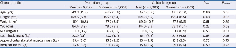
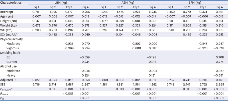
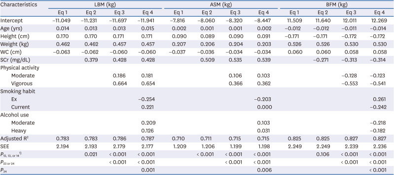
Table 1
Baseline characteristics of study population
![]()
Table 2
Anthropometric prediction equations for lean body mass, appendicular skeletal muscle mass, and fat mass among men
LBM, lean body mass; ASM, appendicular skeletal muscle mass; BFM, body fat mass; Eq, equation; WC, waist circumference; SCr, serum creatinine; SEE, standard error of estimate.
1)P12, 13, or 14 means the P-value of likelihood ratio tests between equation 1 and equation 2, 3, or 4.
![]()
Table 3
Anthropometric prediction equations for lean body mass, appendicular skeletal muscle mass, and fat mass among women
LBM, lean body mass; ASM, appendicular skeletal muscle mass; BFM, body fat mass; Eq, equation; WC, waist circumference; SCr, serum creatinine; SEE, standard error of estimate.
1)P12, 13, or 14 means the P-value of likelihood ratio tests between equation 1 and equation 2, 3, or 4.
![]()
Figs. 1 and 2 show the Bland–Altman plot of LBM, ASM, and BFM in the derivation and validation groups using equation 4 in men and women. These display information about mean differences and agreements. For example, Fig. 1A shows an agreement between LBM and predicted LBM among men in the derivation group. The mean difference was 0.000, implying that the difference between the actual and predicted values by equation 4 was almost zero and suggested a low bias. The limits of agreement were 4.68% outside, meaning that 4.68% of subjects were outside 95% limits of agreement and suggested a moderate agreement. Table 4 depicts the ICC value used to assess the agreement between the novel equation and DXA when utilized in measuring muscle or fat mass. All ICCs were higher than 0.9, which indicated a good agreement between the two methods. In men, the ICCs of the muscle mass equations, such as LBM and ASM, were higher than those of the fat mass equations, like BFM. Conversely, in women, the ICCs of muscle mass equations were lower than those of fat mass.
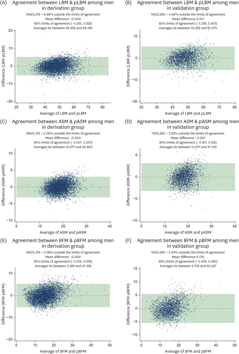
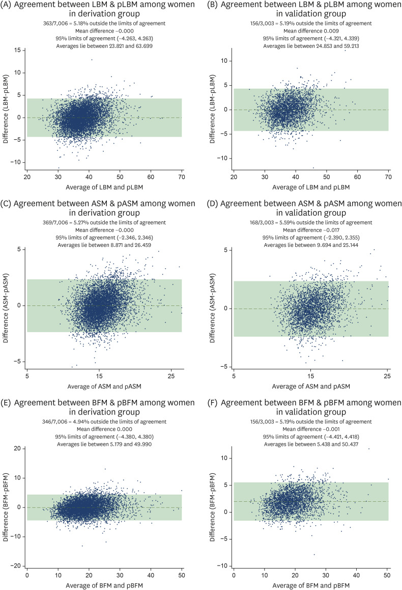
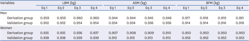
Fig. 1
Bland–Altman plot of the derivation group (left) and validation group (right) for LBM, ASM, and BFM estimates by dual-energy X-ray absorptiometry and prediction equations among men.
LBM, lean body mass; pLBM, predicted lean body mass; ASM, appendicular skeletal muscle mass; pASM, predicted skeletal muscle mass; BFM, body fat mass; pBFM, predicted body fat mass.
![]()
Fig. 2
Bland–Altman plot of the derivation group (left) and validation group (right) for LBM, ASM, and BFM estimates using dual-energy X-ray absorptiometry and prediction equations among women.
LBM, lean body mass; pLBM, predicted lean body mass; ASM, appendicular skeletal muscle mass; pASM, predicted skeletal muscle mass; BFM, body fat mass; pBFM, predicted body fat mass.
![]()
Table 4
Intra-correlation coefficient for agreements of muscle or fat mass between the novel equation and the measured values using dual-energy X-ray absorptiometry
![]()
In cases wherein only BMI is available, and height and body weight are not, we developed and validated the LBM, ASM, and BFM indexes of both men and women (Supplementary Tables 1, 2, 3). The adjusted R2 and ICC of the predicted equations of mass indices were generally lower than that of mass. Supplementary Data 1 shows methods for using anthropometric prediction equations for LBM, ASM, and fat mass among adults.
DISCUSSION
The use of predicted equations for body composition has been previously proposed because imaging modalities, including DXA, CT scan, and MRI, cannot be used even if they are clinically important in measuring body composition. We developed and validated prediction equations to assess LBM, ASM, and BFM among men and women using data obtained with DXA as reference. Considering practicality in the epidemiological settings, we considered four equations that use anthropometric measurements, serum creatinine level, and lifestyle factors. Generally, these predict equations had low bias and moderate agreement ability to assess LBM, ASM, and BFM.
Practical and feasible equations for body composition have been developed; however, only few studies have validated the efficacy of these equations. One study presented two equations that can be used to predict LBM based on measurement obtained via MRI using height and skinfold-corrected upper arm, thigh, and calf girths in 244 adults [10]. The Bland–Altman plot had some proportional error. When using predicted equation, women were over-predicted, and men were under-predicted. Thus, we conducted an independent analysis of prediction equations according to sex. Another study has proposed three equations using ASM measured with DXA as reference and height, body weight, WC, and skinfold thickness and circumference, including those of the triceps, thigh, and calf, among 763 Chinese adults; however, no validation results were obtained, which limited its application in other epidemiological studies [11]. A study conducted in India used a large sample for anthropometric prediction; however, the prediction equation used in that study was limited to Asian population [8]. Furthermore, the Bland–Altman plot had a dumbbell shape, which indicated that women had a lower muscle area and men a higher muscle area and would be proposed separately. A previous study has provided robust validation information for prediction equations [7], but it only included a small number of participants from Asia.
A previous study comparable to our study used DXA as a reference tool in 140,965 participants from the general population included in the National Health and Nutrition Examination Survey [9]. The R2 of LBM and BFM prediction equations based on age, height, weight, and WC ranged from 0.86 to 0.94, and such value was higher than that of our study. Nonetheless, its application to Koreans is limited because the prediction equation was developed based on Western people and some anthropometric values, including circumference of the arm, calf, and thigh (cm) and skinfold-thickness of the triceps and subscapular (mm), are not commonly measured in Korea. Beyond this limitation, there are two statistical limitations to consider: 1) the R2 value was not adjusted and 2) the validation markers would be inappropriate, although suggest the validation information using obesity-related clinical biomarkers included lipid profiles, insulin level, and inflammation marker level [9]. Since the high Pearson's r correlation coefficient of the prediction equation could not guarantee the low bias or error [17], the Bland–Altman plot and ICC have been used to validate the prediction equation [18]. Using a validation study, we confirmed low bias and moderate agreement with the Bland–Altman plot and high reliability with ICC.
Relating to ICC, prediction equations for muscle were higher in men and for fat mass were higher in women, which was related to gender differences in body composition. The differences in body composition between men and women have been extensively studied – men have more lean mass and women have higher fat mass [19]. In particular, the difference is the highest in abdominal adipose tissue, since women have a higher concentration of body fat in the femoral-gluteal region and BFM [20]. For this reason, we suggest separating the two equations according to sex.
The present study had several limitations. First, some anthropometric values, including arm, calf, thigh, and hip circumference and skinfold-thickness of the triceps and subscapular, were not measured in KNHANES. However, these values are less frequently measured in large cohorts. In addition, we considered other factors that might affect body composition, which include serum creatinine level, physical activity, smoking status, and alcohol use. Second, using the Bland–Altman plot, the agreement of prediction equations to mass as measured using DXA was moderate, not high. However, we confirmed that the prediction equations had low bias, high ICC, high adjusted R2, and low SEE, which indicated that these equations can be used in a large cohort. However, caution must be taken when using these prediction equations in a small sample size, or these equations must be used by individuals in the clinical field. Third, because these prediction equations were used in the Korean population, they can be applied to the Asian population; however, caution must be applied when they are used in the Western population.
In conclusion, we developed and validated a series of predict equations for LBM, ASM, and BFM, and their indices using representative national survey. All equations had low bias, moderate agreement based on the Bland–Altman plot, and high ICC, and this result showed that these equations can be further applied to other epidemiologic studies.
 XML Download