From Traditional Statistical Methods to Machine and Deep Learning for Prediction Models

Jun Hyeok Lee; Dae Ryong Kang

doi:10.36011/cpp.2020.2.e6

Abstract

Traditional statistical methods have low accuracy and predictability in the analysis of large amounts of data. In this method, non-linear models cannot be developed. Moreover, methods used to analyze data for a single time point exhibit lower performance than those used to analyze data for multiple time points, and the difference in performance increases as the amount of data increases. Using deep learning, it is possible to build a model that reflects all information on repeated measures. A recurrent neural network can be built to develop a predictive model using repeated measures. However, there are long-term dependencies and vanishing gradient problems. Meanwhile, long short-term memory method can be applied to solve problems with long-term dependency and vanishing gradient by assigning a fixed weight inside the cell state. Unlike traditional statistical methods, deep learning methods allow researchers to build non-linear models with high accuracy and predictability, using information from multiple time points. However, deep learning models cannot be interpreted; although, recently, many methods have been developed to do so by weighting time points and variables using attention algorithms, such as ReversE Time AttentIoN (RETAIN). In the future, deep learning methods, as well as traditional statistical methods, will become essential methods for big data analysis.

INTRODUCTION

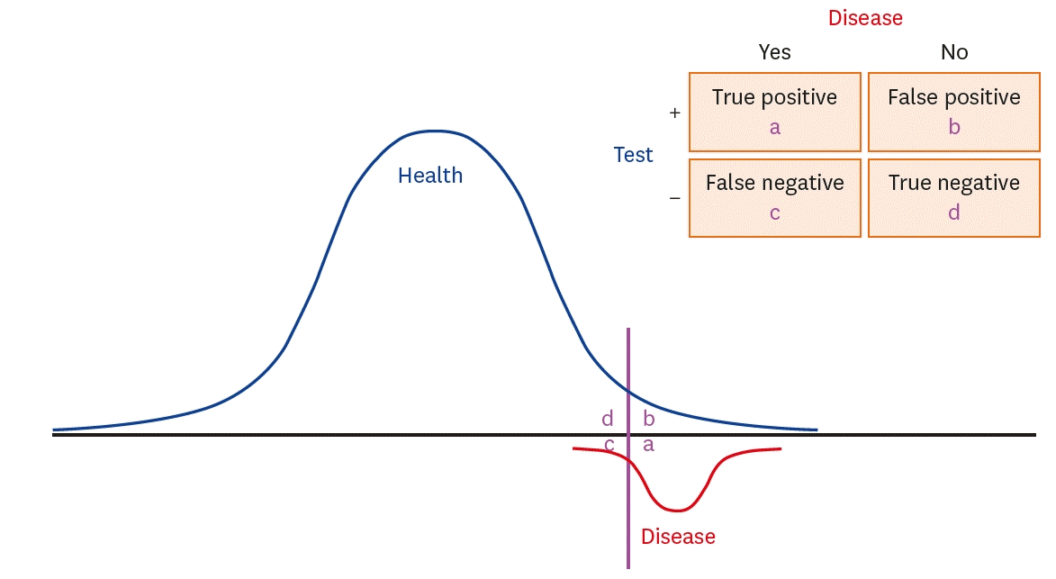
The most important characteristic of a predictive model is its accuracy in distinguishing between healthy and diseased people. Figure 1 depicts an ideal predictive model.

One common method used to develop predictive models based on binary data is logistic regression. However, the major disadvantages of linear regression or logistic regression are its linear nature and its inability to incorporate repeated measures. Many studies have shown that models that use data from multiple time points are more accurate than those that rely on data from a single time point,1-3) and non-linear models built with machine learning are more predictive than linear regression-based models.4) Thus, deep learning methods that integrate both non-linear functions and repeated measures can be used to develop models with high predictive power (Figure 2).

Repeated measures are data collected multiple times for an individual over a study period.5) Observations from repeated measures have been shown to be correlated with each other. To address this with traditional statistical methods, various mixed models with covariance structures have been suggested. Previous studies that applied logistic regression in repeated measures have also relied on methods that use summary statistics, such as the mean, standard deviation, and maximum, as independent variables.1-3) On the other hand, deep learning models can be modeled using actual repeated measures. This paper briefly introduces a representative deep learning method that can be used to incorporate repeated measures in statistical models.

DEEP LEARNING

In the past, it was difficult to calculate weights for various hidden layers. However, improvements in computational speed due to the development of graphics processing units and model optimizations have made it easier to conduct studies on and apply deep learning models. The main deep learning models are convolutional neural networks, recurrent neural networks (RNNs), and deep belief networks.6) This paper focuses on RNNs in the analysis of repeated measures.

RNN

An RNN is a sequence model that processes and delivers information (inputs and outputs) in sequential steps (Figure 3).7) A representative example is a translator. In a translator model, the input is the sentence to be translated (i.e., a word sequence). The translated sentences that correspond to the output are also word sequences. Models designed to process these sequences are called sequence models, and RNNs are the most basic sequence models in deep learning.8)

An RNN can process sequences of an arbitrary length by recursively applying transition functions to hidden states inside the input sequence. At time t, the activation of the hidden state h_t is calculated as a function f of the current input x_t and the previous state h_t−1.

h_{t} = \{\begin{cases} 0 & t = 0 \\ f (h_{t - 1}, x_{t}) & o t h e r w i s e \end{cases}

In general, the affine transformation of x_t and h_t−1 is performed through a non-linear activation function. That is, the input sequence at t receives x_t and f(h_t−1, x_t), which is the hidden state of a previous time.9)

Regarding repeated measures, RNN can reflect the input value of a previous measurement and the input value of a recent measurement. However, RNN models with such structure pose a problem in that the gradient may explode exponentially or disappear in a long sequence of vectors during the training process. These vanishing gradient and long-term dependencies make it difficult for RNN models to learn long sequences.10)11) Hence, long short-term memory (LSTM) models11)12) are used to address these shortcomings.

LSTM

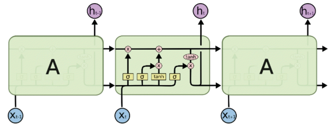
LSTM models are similar to RNNs; however, allowing for a fixed weight inside the cell, gradients can pass through multiple sequences without exploding or losing the slope. LSTM consists of a forget gate, an input gate, and an output gate (Figure 4).8)9)

Each item of the LSTM may be represented as an input gate i_t, a forget gate f_t, an output gate o_t, a cell state c_t, and a hidden state h_t at time t. The first step in LSTM is to decide what information to forget in the cell state. h_t−1, x_t outputs a number between 0 and 1 for cell state c_t−1 through sigmoid a function (σ): 1 indicates keep and 0 indicates remove.

f_{t} = σ (W f ∙ [h_{t - 1},) x_{t}] + b_{f})

The next step is to decide what information to enter in the cell state. The input gate determines the information to update through the sigmoid function (σ), and the tanh function creates a new vector to add to the cell state. These 2 values are used to determine the vector for updating the cell state.

i_{t} = σ (W_{i} ∙ [h_{t - 1},) x_{t}] + b_{i}) c ̃_{t} = \tanh (W_{c} ∙ [h_{t - 1}, x_{t}] + b_{c})

To update a previous cell state c_t−1, the cell state ct of the next time point is generated using f_t of the forget gate and i_t of the input gate.

c_{t} = (f_{t} \times c_{t - 1}) + (i_{t} \times {\tilde{c}}_{t})

Finally, to determine the output vector, the model determines whether to output through sigmoid the function (σ) or to convert the cell state into a non-linear value through the tanh function.

WHY SHOULD WE FOCUS ON MACHINE LEARNING AND DEEP LEARNING?

As repeated measures increase, differences in the accuracy and predictive power of models using a single time point and models using multiple time points increase. There are also limitations with traditional statistical methods in that they must satisfy linearity. In instances of non-linear structures analyzed by traditional statistical methods, the predictive power drops dramatically (Figure 5).

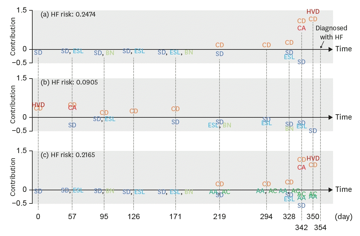
The most significant difference between traditional statistical methods and deep learning is that deep learning models are black-box models that cannot be interpreted. However, research is attempting to address this challenge. One representative example is the ReversE Time AttentIoN (RETAIN) model.13) As shown in Figure 6, a deep learning model can be analyzed by calculating the weight of variables by time (day) and the risk probability of events.

There are also other problems with machine learning and deep learning methods. Since repeated measures from multiple time points are used, the data of a subject cannot be used if there is a missing value at any time point. In addition, because any specific events occur very rarely in big data, it is difficult to match the event cases with corresponding control in the setting. Lastly, as variables can differ at individual time points, setting weights according to importance is crucial.

CONCLUSION

With the vast amounts of data available, single time point and linear models are no longer accurate and predictive. Traditionally, researchers use a single time point or summary statistics in linear regression models. However, with deep learning methods, it is possible to build a predictive model that incorporates data from multiple time points for improved accuracy and greater predictive power. Deep learning methods also make non-linear modeling possible, such that any data structure can be modeled. The shortcomings of deep learning are likely to be improved in the future.

Notes

Conflict of Interest

The authors have no financial conflicts of interest.

Author Contributions

Conceptualization: Kang DR; Investigation: Lee JH; Methodology: Kang DR; Supervision: Kang DR; Visualization: Lee JH; Writing - original draft: Lee JH; Writing - review & editing: Kang DR.

REFERENCES

1. Cho IJ, Sung JM, Chang HJ, Chung N, Kim HC. Incremental value of repeated risk factor measurements for cardiovascular disease prediction in middle-aged Korean adults: results from the NHIS-HEALS (National Health Insurance System-National Health Screening Cohort). Circ Cardiovasc Qual Outcomes. 2017; 10:e004197.

2. Goldstein BA, Navar AM, Pencina MJ, Ioannidis JP. Opportunities and challenges in developing risk prediction models with electronic health records data: a systematic review. J Am Med Inform Assoc. 2017; 24:198–208.

3. Paige E, Barrett J, Pennells L, Sweeting M, Willeit P, Di Angelantonio E, Gudnason V, Nordestgaard BG, Psaty BM, Goldbourt U, Best LG, Assmann G, Salonen JT, Nietert PJ, Verschuren WM, Brunner EJ, Kronmal RA, Salomaa V, Bakker SJ, Dagenais GR, Sato S, Jansson JH, Willeit J, Onat A, de la Cámara AG, Roussel R, Völzke H, Dankner R, Tipping RW, Meade TW, Donfrancesco C, Kuller LH, Peters A, Gallacher J, Kromhout D, Iso H, Knuiman M, Casiglia E, Kavousi M, Palmieri L, Sundström J, Davis BR, Njølstad I, Couper D, Danesh J, Thompson SG, Wood A. Use of repeated blood pressure and cholesterol measurements to improve cardiovascular disease risk prediction: an individual-participant-data metaanalysis. Am J Epidemiol. 2017; 186:899–907.

4. Zack CJ, Senecal C, Kinar Y, Metzger Y, Bar-Sinai Y, Widmer RJ, Lennon R, Singh M, Bell MR, Lerman A, Gulati R. Leveraging machine learning techniques to forecast patient prognosis after percutaneous coronary intervention. JACC Cardiovasc Interv. 2019; 12:1304–11.

5. Lee D, Yoo JK. The use of joint hierarchical generalized linear models: application to multivariate longitudinal data. Korean J Appl Stat. 2015; 28:335–42.

6. Ahn S. Deep learning architectures and applications. J Intell Inf Syst. 2016; 22:127–42.

7. Olah C. Understanding LSTM networks [Internet]. [place unknown]: colah's blog;2015. [cited 2020 Mar]. Available from: https://colah.github.io/posts/2015-08-Understanding-LSTMs/.

8. Lipton ZC, Berkowitz J, Elkan C. A critical review of recurrent neural networks for sequence learning. arXiv 2015:1506.00019.

9. Liu P, Qiu X, Huang X. Recurrent neural network for text classification with multi-task learning. arXiv 2016:1605.05101.

10. Hochreiter S, Bengio Y, Frasconi P, Schmidhuber J. Gradient flow in recurrent nets: the difficulty of learning long-term dependencies. In : Kolen JF, Kremer SC, editors. A Field Guide to Dynamical Recurrent Neural Networks. New York, NY: IEEE Press;2001. p. 237–44.

11. Hochreiter S, Schmidhuber J. Long short-term memory. Neural Comput. 1997; 9:1735–80.

12. Cho K, Van Merriënboer B, Gulcehre C, Bahdanau D, Bougares F, Schwenk H, Bengio Y. Learning phrase representations using RNN encoder-decoder for statistical machine translation. arXiv 2014:1406.1078.

13. Choi E, Bahadori MT, Sun J, Kulas J, Schuetz A, Stewart W. Retain: an interpretable predictive model for healthcare using reverse time attention mechanism. arXiv 2016:1608.05745.

Figure 1.

An ideal model for discriminating between healthy and diseased people.

Figure 2.

Machine and deep learning methods.

ANN = artificial neural network; CNN = convolutional neural network; GAN = generative adversarial network; GRU = gated recurrent unit; LR = logistic regression; LSTM = long short-term memory; RETAIN = ReversE Time AttentIoN; RNN = recurrent neural network; SVM = support vector machine.

Figure 3.

An unrolled Recurrent Neural Network (RNN).

Figure 4.

Structure of long short-term memory.

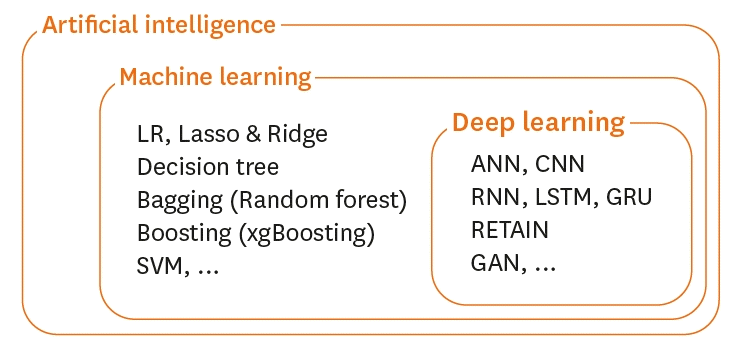
Figure 5.

Graphical illustration of the baselines. As datasets grow in size and complexity, models must evolve accordingly, and logistic regression may no longer be appropriate. In the figure, (A) is a logistic regression model that proceeds directly from x to y; (B) is a multilayer perceptron that proceeds from x to hidden layer v; and (C) has the same structure as a multilayer perceptron. RNNs are structured such that layers circulate with each other. (D and E) are RNN models with attention vectors α_M, and α_R, respectively.

RNN = recurrent neural network.

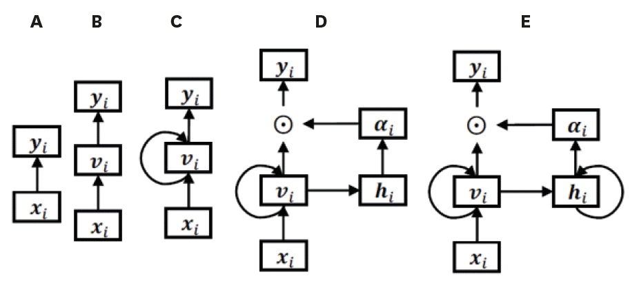
Figure 6.

Temporal visualization of a patient's visit records. The contributions of variables for diagnosis of HF are summarized along the x-axis (time), with the y-axis indicating the magnitude of visit- and code-specific contributions to HF diagnosis.

AA = antiarrhythmic medication; AC = anticoagulant medication; BN = benign neoplasm; CA = coronary atherosclerosis; CD = cardiac dysrhythmia; ESL = excision of skin lesion; HF = heart failure; HVD = heart valve disorder; SD = skin disorder.