Improving Causal Inference in Observational Studies: Interrupted Time Series Design

Kyoung-Nam Kim

doi:10.36011/cpp.2020.2.e2

Abstract

Interrupted time series analysis is often used to evaluate the effects of healthcare policies and interventional projects using observational data. Interrupted time series analysis is one of the epidemiological methods, which are based on the assumption that the trend of the pre-intervention time series, if not intervened, would have the same tendency in the post-intervention period. Time series during the pre-intervention period are used to model a counterfactual situation without intervention during the post-intervention period. The effects of intervention can be seen in the form of abrupt changes in the result level (intercept) due to the intervention and/or changes in the result over time (slope) after the intervention. If the effects of intervention are predefined, the effects of the intervention can be distinguished and analyzed based on the time series analysis model constructed accordingly. Interrupted time series analysis is generally performed in a pre-post comparison using the intervention series. Recently, however, controlled interrupted time series analysis, which uses a control series as well as an intervention series, has also been used. The controlled interrupted time series analysis uses a control series to control potential confounding due to events occurring concurrently with the intervention of interest. Even though interrupted time series analysis is a useful way to assess the effects of intervention using observational data, misleading results can be derived if the conditions for proper application are not met. Before applying the method, it is necessary to make sure that the data conforms to the conditions for proper application.

INTRODUCTION

Although randomized controlled trials are considered as a gold standard to establish causal inference, they are usually not possible for the evaluation of the effectiveness of health care policies and projects performed at population levels.

Interrupted time series design is an increasingly popular epidemiological method, which can improve causal inference in evaluating the effectiveness of interventions using secondary observational data. Interrupted time series studies have been conducted to evaluate the effectiveness of various interventions from air pollution reduction policies1) to new vaccines.2) However, there is a lack of literature that explains the key concepts and outline of the study design for readers who are not familiar with causal inference methods. Therefore, in this paper, the key concepts and outline of interrupted time series design as well as other considerations for application and the use of control are briefly explained.

KEY CONCEPTS AND OUTLINE OF INTERRUPTED TIME SERIES DESIGN

Time series studies use outcomes, such as aggregated numbers of events, that are repeatedly measured (typically at equal intervals) in a specified population. Using time series data, interrupted time series studies aim to evaluate the effectiveness of interventions by comparing time series of outcomes before interventions and those after interventions.

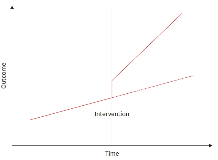
Interrupted time series design has an underlying assumption that trends of time series during the pre-intervention period lasts during the post-intervention period. Therefore, a counterfactual situation without interventions during the post-intervention period is assumed from the extrapolation of time series during the pre-intervention period.3) Hence, in interrupted time series design, the effectiveness of intervention is estimated by comparing actual observations (i.e., time series during the post-intervention period) with the counterfactual situation (i.e., extrapolation of time series during the pre-intervention period and time series during the post-intervention period) (Figure 1).

APPLICATION OF INTERRUPTED TIME SERIES DESIGN

Certain conditions should be satisfied for interventions and outcomes to apply interrupted time series design adequately. First, although it is not necessary for intervention to be implemented at the single time point, timing of the intervention needs to be clearly determined to use interrupted time series design. Second, outcomes need to be affected immediately after intervention or after a pre-specified lag.

Interventions may change outcome levels, slopes, or both. In addition, interventions may also affect outcomes immediately or after a lag period. Before performing analysis, these types of intervention effects (i.e., impact models) need to be defined a priori. It is appropriate that impact models are constructed based on existing literatures and/or assumed mechanisms. If relevant knowledge is lacking, results from the exploratory analysis using alternative data can be used to define impact models. However, constructing impact models using the data which will be employed in the main analyses is not recommended due to the concerns for overfitting.

Segmented regression model in the following form is usually used in the interrupted time series analysis:

Y_t=b₀+b₁×T+b₂×X>_t+b₃×T×X_t (1),

where Y_t represents the outcome of interest at time t, T represents the time since the baseline time point (T=0), X_t is a dummy variable for the intervention at time t (0 for the pre-intervention period and 1 for the post-intervention period), and T×X_t is a multiplicative interaction term for T and X_t.

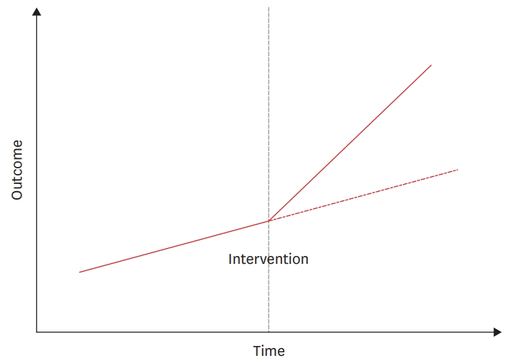
In the above equation assuming that there are both level and slope change (Figure 1), b₂, representing the level change after the intervention, and b₃, representing the slope change after the intervention, are the parameters of interest. In a scenario assuming that there is only level change (Figure 2), which can be modeled with the equation excluding T×X_t from the above Equation 1, b₂, representing the level change after the intervention, is the parameter of interest.

In a scenario assuming that therer is only slope change (Figure 3), which can be modeled with the equation excluding X_t from the above Equation 1, b₃, representing the slope change after the intervention, is the parameter of interest.

If the expected effect size or time points before and/or after intervention are small, the results from the interrupted time series analysis should be interpreted with caution due to the possibility of insufficient power. However, large time points are not always preferred, because historical trend can change over long periods of time, leading to imprecise estimation of the counterfactual situation. Therefore, it is recommended to visually inspect data to determine adequate study period.4)

THE USE OF CONTROL IN INTERRUPTED TIME SERIES ANALYSIS

Although conventional (uncontrolled) interrupted time series design can control for the within-group underlying trend of outcome time series, the possibility of confounding due to time-varying confounders which do not form underlying trend (e.g., interventions and events occurring concurrently with the intervention of interests) remained.5) To decrease this kind of confounding, controlled interrupted time series design, which also uses control series as well as intervention series, can be used.

Control series is defined as a time series which is not exposed to the intervention of interests but is exposed to other interventions and events concurrent with the intervention of interests. It was reported that control series should be selected a priori with a consideration of the sources of possible confounding to prevent data dredging.5)

Intervention series should be assessed using conventional (uncontrolled) interrupted time series analyses before conducting controlled interrupted time series analyses. If effects are found in an intervention series but not in a control series, detected effects are more likely to be due to the effects of intervention. However, if effects are found in both intervention series and control series, observed effects are possibly due to residual confounding by time-varying confounders.

An analytical model for controlled interrupted times series can be summarized in the following equation:

Y_t=b₀+b₁×T+b₂×X_t+b₃×T×X_t+b₄×I+b₅×I×T+b₆×I×X_t+b₇×I×T×X_t (2),

where Y_t represents the outcome of interest at time t, T represents the time since the baseline time points (T=0), X_t is a dummy variable for the intervention at time t (0 for the pre-intervention period and 1 for the post-intervention period), and I is a dummy variable for intervention and control series (0 for control series and 1 for intervention series). In this regression model, b₆ and b₇ are the parameters of interests, which can be interpreted as measures of the effects of intervention.

In addition to the above mentioned method of identifying intervention series and control series with an indicator variable, controlled interrupted time series analyses can be conducted using new variables for the ratio or difference between outcomes of intervention series and control series.

OTHER METHODOLOGICAL CONSIDERATIONS

In time series analyses, outcomes commonly show seasonal patterns, which could induce autocorrelation. Various methods, such as splines or stratification by calendar year, can be applied to control the problems related to seasonality.6) If autocorrelation remains after controlling for seasonality, analytical models, such as autoregressive integrated moving average, can be considered.

Poisson regression is widely used in time series analysis. However, the assumption of equal variance and mean of outcome in poisson regression is easily violated in real data. In many cases, the variance is found to be larger than the mean, which is known as over-dispersion. If there is a concern for over-dispersion, quasi-poisson or negative binomial regression instead of poisson regression can be considered to estimate the standard error correctly.

CONCLUSION

Interrupted time series is becoming increasingly popular as a method for evaluating the effectiveness of interventions. However, interrupted time series analyses can mislead researchers if used carelessly. In order to get correct results from interrupted time series analyses, researchers should understand assumptions of the interrupted time series method and the conditions for proper application.

REFERENCES

1. Yorifuji T, Kashima S, Doi H. Fine-particulate air pollution from diesel emission control and mortality rates in Tokyo: a quasi-experimental study. Epidemiology. 2016; 27:769–78.
2. Lau WC, Murray M, El-Turki A, Saxena S, Ladhani S, Long P, Sharland M, Wong IC, Hsia Y. Impact of pneumococcal conjugate vaccines on childhood otitis media in the United Kingdom. Vaccine. 2015; 33:5072–9.
3. Bernal JL, Cummins S, Gasparrini A. Interrupted time series regression for the evaluation of public health interventions: a tutorial. Int J Epidemiol. 2017; 46:348–55.
4. Lopez Bernal J, Soumerai S, Gasparrini A. A methodological framework for model selection in interrupted time series studies. J Clin Epidemiol. 2018; 103:82–91.