Basic Concepts of Central Limit Theorem
In statistics, a population is the set of all items, people, or events of interest. In reality, however, collecting all such elements of the population requires considerable effort and is often not possible. For example, it is not possible to investigate the proficiency of every anesthesiologist, worldwide, in performing awake nasotracheal intubations. To make inferences regarding the population, however, a subset of the population (sample) can be used. A sample of sufficient size that is randomly selected can be used to estimate the parameters of the population using inferential statistics. A finite number of samples are attainable from the population depending on the size of the sample and the population itself. For example, all samples with a size of 1 obtained at random, with replacement, from the population {3,6,9,30} would be {3},{6},{9}, and {30}. If the sample size is 2, a total of 4 × 4 = 42 = 16 samples, which are {3,3},{3,6},{3,9},{3,30},{6,3},{6,6}...{9,30},{30,3},{30,6},{30,9}, and {30,30}, would be possible. In this way, 4n samples with a size of n would be obtained from the population. Here, we consider the distribution of the sample means.
For example, here is the asymmetric population with a size of 4 as presented above:
The population mean, µ, and variance, σ
2, are:
A simple rando m sampling with replacement from the population produces 4 × 4 × 4 = 4
3 = 64 samples with a size of 3 (
Table 1). The mean and variance of the 64 sample means are 12 (the population mean) and
37.5=σ2n=112.53
, respectively; however, the distribution of the means of samples is skewed (
Fig. 1A).
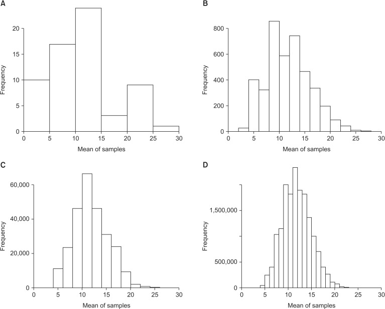 | Fig. 1Histogram representing the means for samples of sizes of 3 (A), 6 (B), 9 (C), and 12 (D).
|
Table 1
Samples with a Size of 3 and Their Means
|
Number |
Sample |
Sample mean |
|
1 |
3 |
3 |
3 |
3 |
|
2 |
3 |
3 |
6 |
4 |
|
3 |
3 |
3 |
9 |
5 |
|
4 |
3 |
3 |
30 |
12 |
|
5 |
3 |
6 |
3 |
4 |
|
6 |
3 |
6 |
6 |
5 |
|
7 |
3 |
6 |
9 |
6 |
|
8 |
3 |
6 |
30 |
13 |
|
9 |
3 |
9 |
3 |
5 |
|
10 |
3 |
9 |
6 |
6 |
|
Truncated |
|
54 |
30 |
6 |
6 |
14 |
|
55 |
30 |
6 |
9 |
15 |
|
56 |
30 |
6 |
30 |
22 |
|
57 |
30 |
9 |
3 |
14 |
|
58 |
30 |
9 |
6 |
15 |
|
59 |
30 |
9 |
9 |
16 |
|
60 |
30 |
9 |
30 |
23 |
|
61 |
30 |
30 |
3 |
21 |
|
62 |
30 |
30 |
6 |
22 |
|
63 |
30 |
30 |
9 |
23 |
|
64 |
30 |
30 |
30 |
30 |

When a simple random sampling with replacement is performed for samples with a size of 6, 4 × 4 × 4 × 4 × 4 × 4 = 4
6 = 4,096 samples are possible (
Table 2). The mean and variance of the 4,096 sample means are 12 (the population mean) and
18.75=σ2n=112.56
, respectively. Compared to the distribution of the means of samples with a size of 3, that of the means of samples with a size of 6 is less skewed. Importantly, the sample means also gather around the population mean. (
Fig. 1B). Thus, the larger the sample size (
n), the more closely the sample means gather symmetrically around the population mean (µ) and have a corresponding reduction in the variance (
σ2n
) (
Figs. 1C and 1D). If
Figs. 1A to 1D are converted to the probability density function by replacing the variable “frequency” with another variable “probability” on the vertical axis, their shapes remain unchanged.
Table 2
Samples with a Size of 6 and Their Means
|
Number |
Sample |
Sample mean |
|
1 |
3 |
3 |
3 |
3 |
3 |
3 |
3 |
|
2 |
3 |
3 |
3 |
3 |
3 |
6 |
3.5 |
|
3 |
3 |
3 |
3 |
3 |
3 |
9 |
4 |
|
4 |
3 |
3 |
3 |
3 |
3 |
30 |
7.5 |
|
5 |
3 |
3 |
3 |
3 |
6 |
3 |
3.5 |
|
6 |
3 |
3 |
3 |
3 |
6 |
6 |
4 |
|
7 |
3 |
3 |
3 |
3 |
6 |
9 |
4.5 |
|
8 |
3 |
3 |
3 |
3 |
6 |
30 |
8 |
|
9 |
3 |
3 |
3 |
3 |
9 |
3 |
4 |
|
10 |
3 |
3 |
3 |
3 |
9 |
6 |
4.5 |
|
Truncated |
|
4087 |
30 |
30 |
30 |
30 |
6 |
9 |
22.5 |
|
4088 |
30 |
30 |
30 |
30 |
6 |
30 |
26 |
|
4089 |
30 |
30 |
30 |
30 |
9 |
3 |
22 |
|
4090 |
30 |
30 |
30 |
30 |
9 |
6 |
22.5 |
|
4091 |
30 |
30 |
30 |
30 |
9 |
9 |
23 |
|
4092 |
30 |
30 |
30 |
30 |
9 |
30 |
26.5 |
|
4093 |
30 |
30 |
30 |
30 |
30 |
3 |
25.5 |
|
4094 |
30 |
30 |
30 |
30 |
30 |
6 |
26 |
|
4095 |
30 |
30 |
30 |
30 |
30 |
9 |
26.5 |
|
4096 |
30 |
30 |
30 |
30 |
30 |
30 |
30 |

In general, as the sample size from the population increases, its mean gathers more closely around the population mean with a decrease in variance. Thus, as the sample size approaches infinity, the sample means approximate the normal distribution with a mean, µ, and a variance,
σ2n
. As shown above, the skewed distribution of the population does not affect the distribution of the sample means as the sample size increases. Therefore, the central limit theorem indicates that if the sample size is sufficiently large, the means of samples obtained using a random sampling with replacement are distributed normally with the mean, µ, and the variance,
σ2n
, regardless of the population distribution. Refer to the
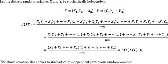
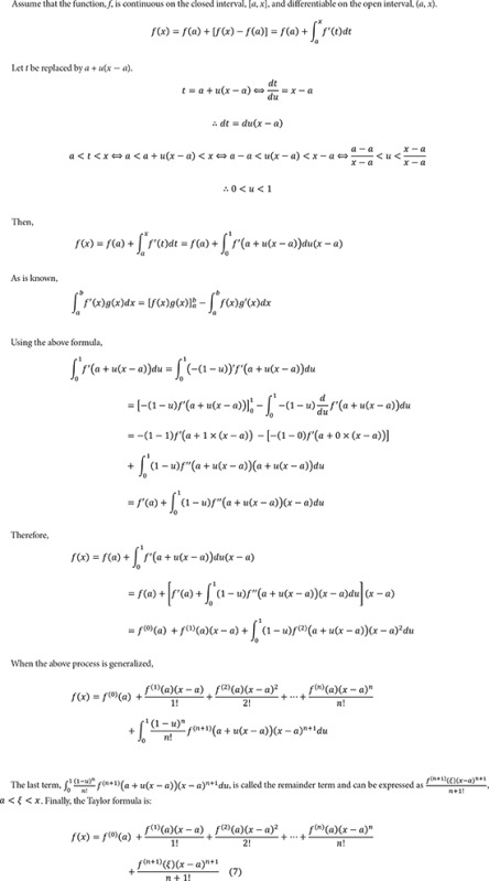
appendix for a near-complete proof of the central limit theorem, as well as the basic mathematical concepts required for its proof.
Go to :

Central Limit Theorem in the Real World
An unbiased, symmetric, 6-sided dice is rolled at random
n times. The probability of rolling the number 3
x times in
n successive independent trials has the following probability density distribution, which is called the binomial distribution:
n: number of in dependent trials (rolling a dice),
x: number of times the number 3 is rolled in each trial,
16
: the probability of rolling the number 3 in each trial, 1 −
16
: the probability of rolling a number other than 3 in each trial.
The mathematical expectation of the random variable, X, (i.e., the number of times that the number 3 is rolled in each trial), which is also referred to as the mean of the distribution, is:
When
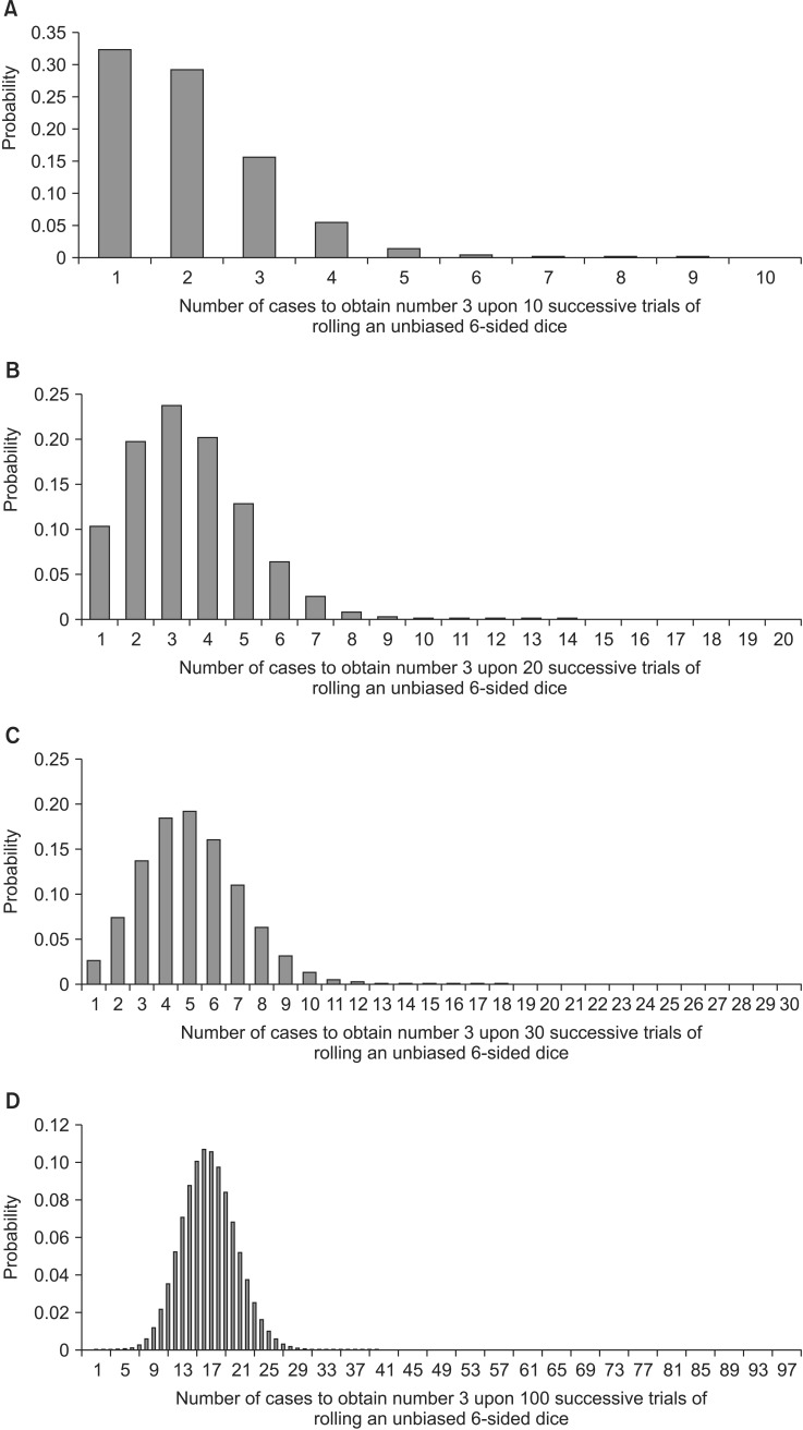
n = 10, the probability has a skewed distribution (
Fig. 2A); however, as
n increases, the distribution becomes symmetric with respect to its mean (
Figs. 2B–2D). As
n approaches infinity, the binomial distribution approximates the normal distribution with a mean,
np, and a variance,
np(1 −
p), where
p is the probability constant for the occurrence of the specific event during each trial.
Go to :

Central Limit Theorem in the Student's t-test
Since the central limit theorem determines the sampling distribution of the means with a sufficient size, a specific mean (X̅) can be standardized
(z=(ˉX-µ)σ√n)
and subsequently identified against the normal distribution with mean of 0 and variance of 1
2. In reality, however, the lack of a known population variance (σ
2) prevents a determination of the probability density distribution.
Xi (i = 1, 2, ..., n): a sample from the population, N: the size of the population, µ: the mean of the population.
Notably, the Student's t-distribution was developed to use a sample variance (S) instead of a population variance (σ2).
xi (i = 1, 2, ..., n): a random sample from the population, n: sample size, X̅: the mean of the samples.
The specific mean (X̅) is studentized
(t=(ˉX-µ)S√n)
and its location is evaluated on the Student's t-distribution, based on the degree of freedom (
n − 1). The shape of the Student's t-distribution is dependent on the degree of freedom. A low degree of freedom renders the peak of the Student's t-distribution lower than that of a normal distribution, although at some points, the tails have higher values than those of the normal distribution. As the degree of freedom increases, the Student's t-distribution approaches the normal distribution. At a degree of freedom of 30, the Student's t-distribution is regarded as equaling the normal distribution [
1]. The underlying assumption for the Student's t-test is that samples should be obtained from a normally distributed population. However, since the distribution of population is not known, it should be determined whether the sample is normally distributed. This is particularly true for small sample sizes. If small sample sizes are normally distributed, the studentized distribution of the sample means is equal to the Student's t-distribution with a degree of freedom corresponding to the sample size. If the small samples are not normally distributed, non-parametric tests should be performed instead of the Student's t-test since they do not require assumptions about the distribution of population. If the sample size is 30, the studentized sampling distribution approximates the standard normal distribution and assumptions about the population distribution are meaningless since the sampling distribution is considered normal, according to the central limit theorem. Therefore, even if the mean of a sample of size > 30 is studentized using the variance, a normal distribution can be used for the probability distribution.
Go to :

 , respectively; however, the distribution of the means of samples is skewed (Fig. 1A).
 , respectively. Compared to the distribution of the means of samples with a size of 3, that of the means of samples with a size of 6 is less skewed. Importantly, the sample means also gather around the population mean. (Fig. 1B). Thus, the larger the sample size (n), the more closely the sample means gather symmetrically around the population mean (µ) and have a corresponding reduction in the variance (σ2n
 ) (Figs. 1C and 1D). If Figs. 1A to 1D are converted to the probability density function by replacing the variable “frequency” with another variable “probability” on the vertical axis, their shapes remain unchanged.
 . As shown above, the skewed distribution of the population does not affect the distribution of the sample means as the sample size increases. Therefore, the central limit theorem indicates that if the sample size is sufficiently large, the means of samples obtained using a random sampling with replacement are distributed normally with the mean, µ, and the variance, σ2n
 , regardless of the population distribution. Refer to the appendix for a near-complete proof of the central limit theorem, as well as the basic mathematical concepts required for its proof.
 : the probability of rolling the number 3 in each trial, 1 − 16
 : the probability of rolling a number other than 3 in each trial.
 and subsequently identified against the normal distribution with mean of 0 and variance of 12. In reality, however, the lack of a known population variance (σ2) prevents a determination of the probability density distribution.
 and its location is evaluated on the Student's t-distribution, based on the degree of freedom (n − 1). The shape of the Student's t-distribution is dependent on the degree of freedom. A low degree of freedom renders the peak of the Student's t-distribution lower than that of a normal distribution, although at some points, the tails have higher values than those of the normal distribution. As the degree of freedom increases, the Student's t-distribution approaches the normal distribution. At a degree of freedom of 30, the Student's t-distribution is regarded as equaling the normal distribution [1]. The underlying assumption for the Student's t-test is that samples should be obtained from a normally distributed population. However, since the distribution of population is not known, it should be determined whether the sample is normally distributed. This is particularly true for small sample sizes. If small sample sizes are normally distributed, the studentized distribution of the sample means is equal to the Student's t-distribution with a degree of freedom corresponding to the sample size. If the small samples are not normally distributed, non-parametric tests should be performed instead of the Student's t-test since they do not require assumptions about the distribution of population. If the sample size is 30, the studentized sampling distribution approximates the standard normal distribution and assumptions about the population distribution are meaningless since the sampling distribution is considered normal, according to the central limit theorem. Therefore, even if the mean of a sample of size > 30 is studentized using the variance, a normal distribution can be used for the probability distribution.


 PDF
PDF Citation
 Print
Print



 XML Download