Introduction
Data science and machine learning (ML) are topics that have received enormous attention in recent years. Their strongest driving force seems to be in the explosion of data, both in size and scope. Several success stories of applying ML technology have increased worldwide investment in this area [
1], and medicine is no exception.
As with other medical fields, ML is revolutionizing anesthesiology research. Unlike classical research methods that are largely inference-based, ML is more geared toward making accurate predictions [
2]. Medical textbooks are full of well-validated risk factors but only few well-validated predictive systems.
Being aware of this limitation, medical researchers and societies have strived to create effective predictive algorithms [
3]. A widely employed method for clinical prediction is the development of a risk scoring system. The researcher cleverly puts together previously known risk factors to yield a single output score. The Child–Pugh score is a well-known example. Based on five clinical measures of total bilirubin, serum albumin, prothrombin time, ascites, and hepatic encephalopathy, a score ranging from 5 to 15 is calculated. Ranges of 5 to 6, 7 to 9, and 10 to 15 points are equivalent to the Child–Pugh classes of A, B, and C, respectively. This system was first proposed in 1964 by the surgeon Charles Gardner Child [
4], and modified by Pugh et al. in 1972.
A scoring system is a big step forward toward implementing an actual prediction algorithm based on multiple factors. However, the methods of constructing such a system have been rather haphazard and based on trial and error. ML has much to offer in this regard.
Much of the recent hype about artificial intelligence (AI) and ML mainly centers around a specific ML algorithm called deep learning. To a newcomer in this field, it might seem that AI and deep learning are equivalent terms. However, AI, as an academic field, has existed for a long time and deep learning (a.k.a. multi-layer perceptron, the old-fashioned term) is one of its many research topics. Most of its important theoretical development already took place in the mid-twentieth century but its enormous potential was unrecognized for a long time.
The landscape of ML can be envisioned as fundamentally consisting of three large categories:
supervised learning, unsupervised learning, and
reinforcement learning (
Fig. 1). Algorithms that constitute each of these categories are diverse, and deep learning is merely one of them. Deep learning is special in certain aspects and supersedes all other algorithms when dealing with tasks related to images, videos, sounds, and machine translation. However, deep learning is occasionally overstated in its capability and misconceived as a magic wand. It is necessary to gain a clear overview of the entire field of ML before digging deeper into any specific algorithm.
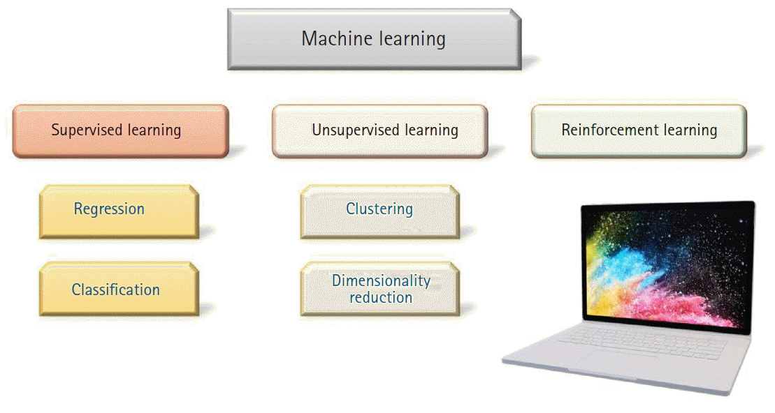 | Fig. 1.Machine learning (ML) Landscape. ML algorithms can roughly be divided into three categories – Supervised learning, unsupervised learning, and reinforcement learning. Our focus will primarily be on supervised ML algorithms. 
|
This article will primarily deal with data science and ML as applied to anesthesiology using electronic health records (EHRs). Owing to their retrospective character, the main limitation of EHR-based studies is the difficulty of establishing causal relationships. However, the low cost and rich information content provide great potential to uncover hitherto unknown correlations. Such correlations can generate hypotheses to be tested through prospective clinical trials.
Go to :

Basic concepts of ML
ML is a field of AI concerned with developing algorithms and models to perform prediction tasks in the absence of explicit instructions. ML algorithms build a predictive model based on some training data that consist of features. A good understanding of these terms is crucial in acquiring a firm grasp of ML. Hereafter, important terms will be highlighted in italics.
Data
The data D in a ML task is expressed using a matrix
[x11⋯x1m⋯⋯⋯xn1⋯xnm]. The
ith row of X is called an ith
instance of D. The
jth column of X, on the other hand, is called a
jth feature of D. Throughout this review, we will use a well-known dataset in the ML community (the Pima Indian diabetes dataset), originally from the National Institute of Diabetes and Digestive and Kidney Diseases (
https://www.niddk.nih.gov/), which consists of 768 subjects and 8 features. These features are as follows: number of prior pregnancies, plasma glucose concentration (glucose tolerance test), diastolic blood pressure (mmHg), triceps skin fold thickness (mm), 2-h serum insulin (mu U/ml), body mass index (BMI), diabetes pedigree function, and age (
Table 1). The objective is to predict whether the patient is diabetic, based on the values of these features.
Table 1.
Pima Indians Diabetes Dataset with 768 subjects and 8 features
|
Pregnancies (number) |
Glucose (mg/dl) |
Blood pressure (mmHg) |
Skin thickness (mm) |
Insulin (mu U/dl) |
BMI (kg/m2) |
Diabetes pedigree function |
Age (yr) |
Outcome |
|
6 |
148 |
72 |
35 |
0 |
33.6 |
0.627 |
50 |
1 |
|
1 |
85 |
66 |
29 |
0 |
26.6 |
0.351 |
31 |
0 |
|
8 |
183 |
64 |
0 |
0 |
23.3 |
0.672 |
32 |
1 |
|
1 |
89 |
66 |
23 |
94 |
28.1 |
0.167 |
21 |
0 |
|
0 |
137 |
40 |
35 |
168 |
43.1 |
2.288 |
33 |
1 |
|
5 |
116 |
74 |
0 |
0 |
25.6 |
0.201 |
30 |
0 |
|
3 |
78 |
50 |
32 |
88 |
31 |
0.248 |
26 |
1 |
|
10 |
115 |
0 |
0 |
0 |
35.3 |
0.134 |
29 |
0 |
|
2 |
197 |
70 |
45 |
543 |
30.5 |
0.158 |
53 |
1 |
|
8 |
125 |
96 |
0 |
0 |
0 |
0.232 |
54 |
1 |
|
4 |
110 |
92 |
0 |
0 |
37.6 |
0.191 |
30 |
0 |
|
10 |
168 |
74 |
0 |
0 |
38 |
0.537 |
34 |
1 |
|
10 |
139 |
80 |
0 |
0 |
27.1 |
1.441 |
57 |
0 |
|
1 |
189 |
60 |
23 |
846 |
30.1 |
0.398 |
59 |
1 |
|
5 |
166 |
72 |
19 |
175 |
25.8 |
0.587 |
51 |
1 |
|
7 |
100 |
0 |
0 |
0 |
30 |
0.484 |
32 |
1 |
|
0 |
118 |
84 |
47 |
230 |
45.8 |
0.551 |
31 |
1 |
|
7 |
107 |
74 |
0 |
0 |
29.6 |
0.254 |
31 |
1 |
|
1 |
103 |
30 |
38 |
83 |
43.3 |
0.183 |
33 |
0 |

Task
A task is a problem we want to solve—the most common ones being classification and regression.
In classification, the target variable (or label) is an element of a countable set S = {C1, …, Ck}. In our running example, S has two elements {diabetes mellitus (DM) absent, DM present}. For notational convenience, we assign 0 and 1 to each element, respectively. The role of the ML algorithms is to discover an appropriate mapping from the features to {0, 1}. Such a mapping is called a model.
In regression, the target variable is a real number (often restricted to be positive). The task, therefore, is to construct a model that generates a real-numbered prediction that is as similar to the target variable as possible.
Model and parameters
A model takes in features as inputs, performs some logical or mathematical operations, and generates an output. For example, a model can consist of a set of if-then rules such as:
If age > 60 yr and BMI > 30 then output = 1 else output = 0
The cutoff values, 60 yr and BMI of 30, are called parameters of the model. Given the model, optimal parameter values must be found such that the outputs are as close to the actual target values. For various reasons, ML algorithms instead try to find parameters that yield the least dissimilar outputs to the target variables. The metric of dissimilarity is called a loss function. Depending on the specific task, different loss functions are chosen. For our classification task, we could imagine assigning a value of +1 if there is a mismatch between the output and the target variable, and 0 otherwise. The sum of the assigned values of all instances divided by the number of instances is then defined as the expected loss. The parameters that yield the smallest magnitude of this value become the solution of this task.
The above-mentioned set of if-then rules can be combined into a tree, yielding a tree model (
Fig. 2). The
decision tree algorithm is a popular ML sequence that provides an intuitive framework to make classifications and decisions. Often, multiple trees are generated on random subsets of the original data. The decisions of the individual trees are then combined to generate the final prediction. This algorithm is known as the
random forest algorithm [
5].
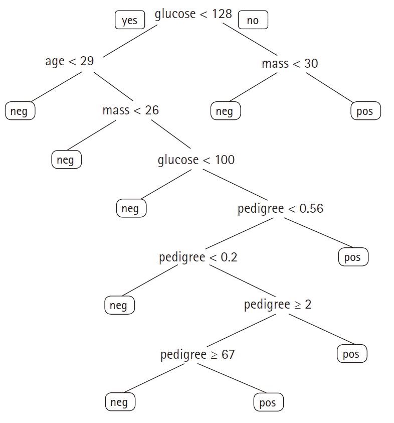 | Fig. 2.A decision tree to predict the presence of diabetes based on the Pima Indians Diabetes dataset (glucose: serum glucose [mg/dl], age [yr], mass: body mass index [kg/m2], pedigree: diabetes pedigree function). neg: negative, pos: positive. 
|
The practical use of ML involves choosing the right model to apply to data. There is no single model that works best for every task, a fact that is referred to as the
no free lunch theorem of ML [
6]. It is usually required to try multiple models and find one that works best for a task. This trial and error process lies at the heart of ML artistry. The list of commonly used ML algorithms is as follows:
Researchers generally fit different ML algorithms to data and compare the predictive performances. The one that yields the highest performance is generally chosen as the final predictive model.
A specific approach called the
ensemble method is noteworthy. As the term implies, this method combines several ML algorithms into a single model, and can be approximately divided into two types:
sequential and
parallel methods. In the former, the base learner is trained sequentially, each time assigning more weights to previous errors. Prototypical algorithms are
AdaBoost and
Gradient Boost [
7,
8]. Parallel methods, on the other hand, combine learners that have been trained independently. The above-mentioned random forest algorithm is the prototype.
Loss functions
The choice of the loss function is intricately related to the task and the model type.
In regression, the loss function is formulated so that it reflects the expected error. The most commonly used loss function is the mean squared error (MSE), defined as 1n∑(yi-f(Xi))2, where, yi and f(Xi) are the target variable and the model output of the ith instance, respectively. Root-mean-square error (RMSE), which is defined simply as √MSE, is also widely used. The latter has an advantage that the scale of the error is the same as that of the target variable. It is possible to state that the model generates outputs with an error margin of ε (%), where, ε = 100(%)×√MSE/(mean prediction).
In classification tasks, the model output is a number between 0 and 1, often interpreted as the probability of the target yi being positive. Binary cross entropy, defined as –[yilogpi + (1-yi)log(1-pi)], where, pi is the model output for the ith instance, is widely used as the loss function.
Optimization algorithms are used to search the parameter space of a given model so that the loss function is minimized. There are various algorithms, the most common one being based on calculating the
gradient of the loss function. It is an iterative search algorithm where the parameter values are updated every time based on the calculated gradient of the current parameter estimates. A gradient is a multivariate extension of a
derivative. Since the loss function, L, is a function of its parameters p, changing the values of p results in changes in L. Intuitively, changing p in the direction that most sensitively affects L is likely to be an effective search strategy. To illustrate this idea more vividly, imagine a landscape where the value of L is plotted along the vertical axis and the parameters (restricted to two-dimensional for demonstrative purposes) on the horizontal plane (
Fig. 3). Supposing that a certain agent is riding along the ridges of the loss function surface, searching for its deepest valley, starting from any arbitrary point on the surface, a plausible search strategy would be to look around and descend down the path with the steepest slope. A tangent with the steepest slope, the derivative in a univariate problem, is the gradient. Repeating such a search often results in the agent ending up in one of the valleys, which is a potential solution to the search task. Unfortunately, the gradient-based search strategy does not guarantee a globally optimal solution when applied to a loss function surface with multiple peaks and valleys, as shown in
Fig. 3. Methods to circumvent this limitation do exist (such as introducing a momentum, starting the search from multiple initial parameter values, adopting a stochastic component, and so on) but none of them definitely solve the problem (other than the brute-force strategy of searching all possible parameter combinations). For more information, refer to [
9].
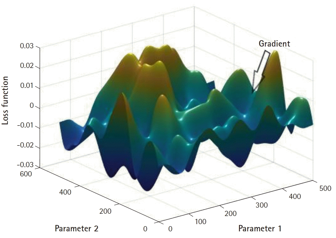 | Fig. 3.A hypothetical landscape illustrating the relationship between the loss function and the parameters. 
|
Overfitting and underfitting
An important limitation associated with minimizing a loss function given a set of features, target variables, and a model is that this does not necessarily minimize the difference between f(X) and the true signal ˜Y. The optimized prediction ˆY = f(X) may be closest to Y = ˜Y + ε (where, ε is a random error) but not to ˜Y. This phenomenon is given an infamous name called overfitting in ML literature.
To avoid overfitting, one often keeps a separate dataset with an identical signal ˜Y but different random error ε’. Overfitting can be detected by comparing the loss function based on the original dataset with that calculated using the separate dataset. A significant difference between the two loss functions indicates that the parameters are fitting the random error ε.
Training, validation, and test datasets
In ML nomenclature, the original dataset used to optimize the parameters is called the training dataset, and a separate dataset used for detecting overfitting is called the test dataset. Hereafter, training and test datasets will be denoted as Tr and Te, respectively. It is customary in ML practice to randomly split D into Tr and Te. The split ratio is often chosen such that the size of Tr is greater than Te.
While this practice partly safeguards against overfitting, repeated bouts of training can lead to the overfitting of Te as well. Hence, Tr is generally split yet again into (real) training and
validation (V)
datasets (
Fig. 4).
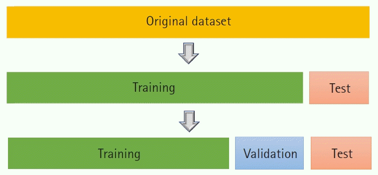 | Fig. 4.Splitting of the dataset into training, validation, and datasets. Model comparison is done using the validation dataset. Predictive performance of the final model is assessed using the test dataset. 
|
In analogy, V serves the purpose of practice exams. Optimization on Tr is followed by validation on V. When there is room for improvement, either a different model is chosen, or model hyper-parameters are modified. The procedure of training the new or modified model is repeated until a satisfactory result on V is achieved. The final predictive model is then validated using Te. If the predictive performance on Te is comparable to that on Tr, the model is then accepted and used.
A variant of this procedure, called k-fold cross-validation, is also widely used. First, Tr is partitioned into k chunks (often of equal or similar sizes). One of the k chunks is defined as V and the rest as Tr. Then, the predictive performance on V is assessed, and this procedure is repeated on all possible allocations of V and Tr. Finally, the k assessment scores from the k validation runs are averaged to yield the mean performance index. Models that improve the mean performance index are chosen.
While splitting D into Tr and V, and Te is the standard method to tackle overfitting, one should always try to directly incorporate the data generating mechanism if possible. For example, to predict the concentration of an anesthetic drug that is known to be eliminated from the kidney by first order kinetics, it would be a better choice to use a pharmacokinetic model C(t) = C(0)e(-kt) (k: elimination rate constant) than to use a high degree polynomial C(t) = C(0) + β1t + + β2 t2 … + βp tp. The latter function can undoubtedly generate outputs that match the observed concentrations given a sufficiently high degree p. However, this model would be prone to overfitting the data.
Feature selection
Not all features are informative in predicting the target. Returning to our running example of the Pima Indians Diabetes dataset, supposing that in addition to the 8 features, we are given the favorite movie genre of the subjects. This additional feature, however, is unlikely to improve predictive performance because movie preference is not related to the development of diabetes in any meaningful way.
A more serious problem occurs when so-called collinear features are present. Suppose the data consist of weights measured in kilograms and pounds as two distinct columns (i.e., features). If a classification model is built using both features, the optimization algorithm would fail to converge. This is because the relative contribution of each of the two features to the model output cannot be uniquely determined.
First, the investigator must inspect the features manually and filter them based on domain knowledge. Here, features, such as patient names (which have no information in predicting the target of our interest) are excluded.
After manual filtering of the features, feature selection algorithms can be applied. There are basically three different classes of such algorithms: (1) stepwise selection methods that iteratively incorporate the “best” feature at each step, (2) dimensionality reduction techniques that extract the most important components to be used as new features, and (3) regularization or shrinkage methods that penalize large parameter values during the optimization process.
The stepwise selection method is an umbrella term for all approaches that selects the one best feature at a time, evaluates the gain in predictive performance, and then decides whether it should be included in the model (
Fig. 5). While stepwise selection algorithms do not always provide the optimal solution, they are easily understandable and simple to implement.
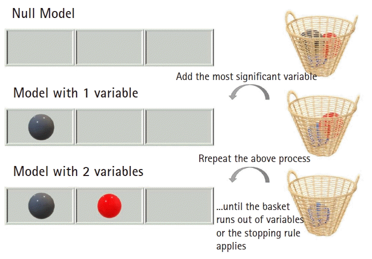 | Fig. 5.The stepwise selection procedure. Each time, the most significant variable is incorporated into the prediction model. Such a selection process is repeated over all candidate variables until no more candidates exist or the algorithm hits a predefined stopping rule. 
|
Dimensionality reduction techniques eliminate collinearity by lumping correlated features. For example, given features of height and weight, a new feature of BMI can be calculated from the two. Replacing height and weight with BMI reduces the number of features and at the same time solves the problem of feature collinearity. One of the most popular dimensionality reduction methods is the
principal components analysis. Given multiple features, the method identifies the principal components that retain as much of the original variance as possible. For more information on this particular method, refer to [
10].
Lastly, regularization controls the magnitude of regression coefficients. This is based on the premise that large magnitude coefficients (in the order of tens to thousands) are unlikely. From a Bayesian point of view, regularization is equivalent to imposing a null hypothesis of non-significance to all features (i.e., zero coefficient). Large coefficients that deviate from zero are thus penalized in the calculation of the loss function. The three widely used regularization schemes are called
LASSO,
Ridge, and
ElasticNet [
11]. A more interested reader is referred to a review article that specifically deals with various feature selection methods [
12].
Multilayer neural network algorithms, so-called deep learning, can automatically extract useful features from the raw input. This is one of the great advantages of this algorithm and has contributed to its high popularity.
Assessment of predictive performance
Training models is important; however, assessing their performance and selecting the best model is perhaps even more important. This is particularly true for medical researchers since ML engineers can be hired to do the computational work but judging the overall quality of the work remains the responsibility of the principal investigator.
A better model is the one that makes fewer errors. In regression, such a model is the one associated with a lower MSE. In classification, a model with a higher accuracy, defined as the fraction of correctly classified instances, might be used. However, more subtle complications arise when there is an imbalance among the classes. Referring to our running example, suppose that 99% of the subjects were diabetic. In such a case, simply predicting all subjects as diabetic would achieve an accuracy score of 99%.
A
confusion matrix is a table showing the frequencies of true positives (TP), false positives (FP), true negatives (TN), and false negatives (FN) (see
Table 2).
Table 2.
|
Prediction = 0 |
Prediction = 1 |
|
Actual target = 0 |
TN |
FP |
|
Actual target = 1 |
FN |
TP |

Several important metrics are defined based on the values of the confusion matrix:
(i) Sensitivity (a.k.a. recall, true positive rate) = TP(FN+TP)
(ii) Specificity (a.k.a. selectivity, true negative rate) = TN(TN+FP)
(iii) Precision (a.k.a. positive predictive value) = TP(FP+TP)
(iv) Negative predictive value = TN(TN+FN)
The most important concept related to the application of the confusion matrix is the tradeoff between sensitivity and specificity. The most sensitive algorithm is the one that predicts everything positive, i.e., the sensitivity is 100%. Such a simple method guarantees that the algorithm classifies every positive instance correctly (all instances are classified as positive anyway). However, the price paid is that no negative instance is classified correctly, yielding a specificity of 0%. Since the definition of positives and negatives is arbitrary, it is easy to imagine that by flipping their definitions, a 100% specificity can be achieved at the cost of 0% sensitivity.
As an analogy, an anticancer drug that kills all cells will certainly eradicate all cancer cells. The sensitivity is 100%. However, since this drug would kill off all healthy cells as well (i.e., specificity 0%), such a drug will never make it to the clinic.
One must find an optimal point where both sensitivity and specificity are acceptable for practical use. Evidently, this is no longer a mathematical problem. If sensitivity is more important (e.g., cancer diagnosis), the cost associated with the lower specificity can be tolerated.
Now, suppose model A achieves 90% sensitivity and 10% specificity while model B achieves 10% sensitivity and 90% specificity. Which of the two models is the better?
The widely adopted solution is to first draw a curve called a receiver operating characteristic (ROC) curve, which is created by plotting sensitivity against 1 – specificity, and then calculate the area under the curve (AUC). An ideal algorithm that achieves 100% sensitivity and 100% specificity would be associated with an AUC of 100%, which is the maximum score achievable. A random guess, due to the tradeoff between sensitivity and specificity, would satisfy the following equality:
Sensitivity + Specificity = 100%
The ROC curve is then a straight line with slope of unity that passes through the origin, and its AUC is 50%
Fig. 6A).
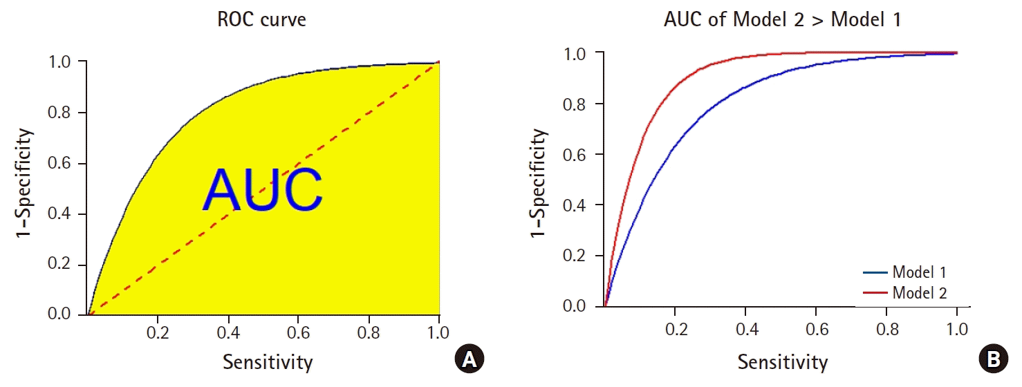 | Fig. 6.The receiver operating characteristic (ROC) curve and the area under the curve (AUC). (A) The yellow shaded area corresponds to the AUC. The dotted red line corresponds to the ROC curve of a random guess algorithm. (B) A model associated with a higher AUC is generally taken to be a better model. 
|
Most predictive models have AUC values that fall between these two extremes: 50% and 100%. Model selection, therefore, is often carried out by comparing the AUC of ROC curves
Fig. 6B).
The use of AUC, however, is not without problems. Lobo et al. [
13] recommend against the use of AUC for the following reasons: it ignores the predicted probability values, summarizes the test performance over regions of the ROC space in which one would rarely operate, weights omission and commission error equally, does not inform about the distribution of model errors, and most importantly, the total extent to which models are carried out highly influences the rate of well-predicted absences and the AUC scores.
A widely used alternative to the AUC is the F1 score, defined as the harmonic mean of precision and sensitivity:
Notwithstanding these issues, AUC is currently the standard method widely used for model comparison and assessment of predictive performance.
Summary
Supervised ML requires that the data be expressed as a matrix. Each row corresponds to an instance of the learning material, while each column represents the values of the different features. The matrix is subsequently fed into a suitable model that consists of tunable parameters. The machine carries out the learning process by minimizing a predefined loss function. All loss functions reflect the degree to which the model outputs differ from the true values, playing the role of a supervisor.
Different models are trained on Tr and their predictive performances assessed on V. A metric such as the AUC of the ROC curve must be chosen prior to the analysis as the model selection criterion. Models are then compared using this metric, where the model yielding the highest (or lowest) value is selected as the final model. The predictive performance of the final model is judged using Te. If the performance reasonably matches that of Tr and V, one can be assured that overfitting has not occurred to any significant degree. The final model is then deployed as a real-world application.
Go to :


 PDF
PDF Citation
 Print
Print


 XML Download