Covariates violating the proportional hazard assumption in a CPH model should be adequately adjusted. This section introduces a stratification and time-dependent Cox regression to deal with covariates violating the proportional hazard assumption.
R codes for stratified Cox proportional hazard model
In the previous CPH modeling, the variable ‘Inopioid’ violated the constant hazard assumption based on the Schoenfeld residual test (
Fig. 6). Here, ‘Inopioid’ is a continuous variable that records the dose of intraoperatively used opioid. To apply a stratified CPH modeling, continuous variables should be converted into categorical variables. For convenience, the following is a code that converts ‘Inopioid’ into a categorical variable of 0 or 1, when not used or used, respectively.
##### Stratified Cox regression
### Add categorical variables from Inopioid
PONV.raw <- transform(PONV.raw,
Inopioid_c = ifelse(
Inopioid == 0, 0, 1))
head (PONV.raw)
According to this, the categorical variable ‘Inopioid_c’ is recorded as 0 or 1 and is newly added to the dataset (
Table 7).
Table 7.
PONV.raw Added a New Categorical Variable ‘Inopioid_c’ from the Variable ‘Inopioid’
Results of ‘head (PONV.raw)’
|
|
No |
Antiemetics |
Age |
Wt |
Inopioid |
Time |
PONV |
Survobj |
Inopioid_c |
|
1 |
1 |
0 |
48 |
78.5 |
0 |
4 |
0 |
4+ |
0 |
|
2 |
3 |
0 |
54 |
88.3 |
100 |
21 |
0 |
21+ |
1 |
|
3 |
4 |
0 |
22 |
49.4 |
0 |
14 |
0 |
14+ |
0 |
|
︙ |
︙ |
︙ |
︙ |
︙ |
︙ |
︙ |
︙ |
︙ |
︙ |

Next, the code for a stratified CPH model is as follows:
### Stratified Cox proportional hazard modeling
cph.strata <- coxph (Surv(Time, PONV == 1)
~ Antiemetics + strata(Inopioid_c)
, data = PONV.raw)
summary (cph.strata)
ggsurvplot(survfit(cph.strata)
, data = PONV.raw
, risk.table = TRUE
, palette = c("black","black")
, linetype = c("solid","dashed")
)
par( mfrow = c(1,1))
plot (survfit(cph.strata)
, fun = "cloglog"
, main = "Antiememtics"
)
sf.residual.strata <- cox.zph(cph.strata)
print(sf.residual.strata)
plot(sf.residual.strata)
abline (h = coef(cph.strata)
, lty = "dotted"
, lwd = 1)
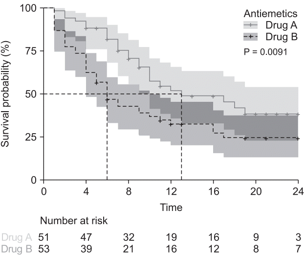
This code outputs a stratified CPH model by controlling ‘Inopioid_c’ (
Table 8). The command ‘ggsurvplot’ provides survival curves of two strata and prints the LML plot using the last ‘plot’ command (
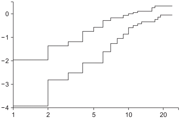
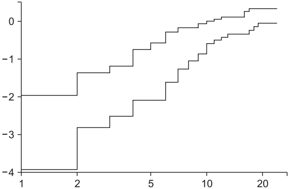
Fig. 7). The Schoenfeld residual test using a ‘cox.zph’ command reveals that ‘Antiemetics’ violates the proportional hazard assumption (rho = −0.265, chisq = 4.26, P = 0.039, shown in
Fig. 8). It is possible to obtain an adequate CPH model by stratifying ‘Inopioid’ and ‘Antiemetics’, although the interpretations may be complex because it is difficult to integrate the comparison results among all strata.
Fig. 7.
Examples of the stratified Cox proportional hazard model and corresponding LML plot. (A) Survival curves of estimated stratified Cox proportional hazard model. Stratification is achieved using the categorical variable ‘Inopioid_c’. (B) Log-minus log plot for evaluation of proportional hazard assumption against two antiemetics. Note that a non-parallelism of below 2 h is not assured, whereas the overall curves are roughly parallel without crossing.
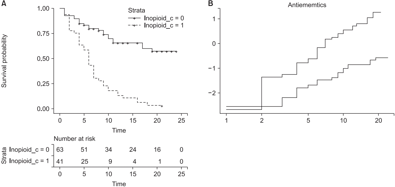

Fig. 8.
Schoenfeld residual test for the stratified Cox proportional hazard model. For the covariate ‘Antemetics’, the probability was estimated as 0.039, and a violation of the proportional hazard assumption was strongly suggested under the controlled covariate ‘Inopioid’ (the dotted horizontal line shows the estimated coefficient of ‘Antiemetics’).
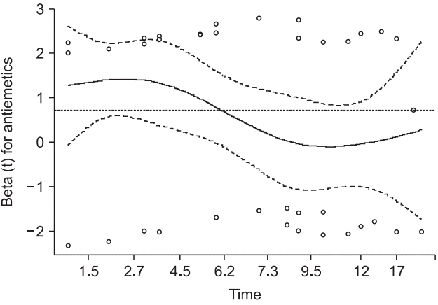
Table 8.
Results of Stratified Cox Proportional Hazard Model. Stratification with ‘Inopioid_c’
Call: coxph(formula = Surv(Time, PONV == 1) ~ Antiemetics + strata(Inopioid_c), data = PONV.raw)
|
n = 104, number of events = 63
|
|
coef |
exp(coef) |
se(coef) |
z |
Pr(>|z|) |
|
|
Antiemetics |
0.7282 |
2.0714 |
0.2625 |
2.774 |
0.00553** |
|
|
--- |
|
|
|
|
|
|
|
Signif. |
codes: |
0 ‘***’ |
0.001 ‘**’ |
0.01 ‘*’ |
0.05 ‘.’ |
0.1 ‘’ |
|
|
exp(coef)
|
exp(-coef)
|
Lower .95
|
Upper .95
|
|
|
|
|
Antiemetics |
2.071 |
0.4828 |
1.238 |
3.465 |
|
|
|
Concordance |
|
= 0.634 |
(se = 0.034) |
|
|
|
|
Rsquare |
|
= 0.074 |
(max possible = 0.979) |
|
|
|
|
Likelihood ratio test |
|
= 7.96 |
on 1 df, P = 0.005 |
|
|
|
|
Wald test |
|
= 7.7 |
on 1 df, P = 0.006 |
|
|
|
|
Score (logrank) test |
|
= 8.03 |
on 1 df, P = 0.005 |
|
|
|
Time-dependent Cox regression
Most clinical situations change over time, and the variables affected by a specific treatment also change even when the treatment remains constant during the observation period [
13]. For example, consider an analgesic having a toxic effect on the hepatobiliary function for patients with chronic pain. A periodic liver function test will be crucial, and all laboratory results will vary for every follow-up time. The administration dose may also vary according to the laboratory results or analgesic effects. Moreover, the laboratory results may not be valid after the patients are censored or after an event occurs. These variables are common in clinical practice, and the existence of time-dependent variables should be considered and checked before starting the data collection for survival analysis. If an adequate measurement method is developed, a time-dependent covariate Cox regression will be possible. Another type of time-dependent variable is a covariate with a time-dependent coefficient [
14]. If the analgesics mentioned above produces a level of tolerance, its effect decreases over time. This indicates that the risk of breakthrough pain occurrence may be higher as time passes, which apparently violates the proportional hazard assumption. In this case, the effect of the analgesics can be included in the survival function, which is expressed as a covariate with a coefficient of the function of time.
As mentioned above, a time-dependent covariate is incorporated into the analysis as a single value according to the repeated observation intervals. For example, a patient under analgesics medication takes an initial liver function test, the results of which show 40 IU/L and 100 IU/L after four weeks with continued pain and 130 IU/L at eight weeks with pain, whereas at 12 weeks after analgesics administration, the pain is subsided and medications are discontinued without a further laboratory test. The laboratory data input for the time-dependent covariate are 40 until 4th weeks without an event, 100 from 4th to 8th weeks without an event, 130 from 8th to 12th weeks, and an event occurs at 12th weeks.
Clinical studies in the area of anesthesiology often include variables related to the response or effect of a specific treatment or medication. Depending on the characteristics and measurement methods of the variables, once a specific treatment or medication is applied, their effects are gradually decreased over time or delayed until the onset time. The effects of treatment or medication changes over time, the coefficient of these effects can be expressed as a time function, and for Cox regression, a step function is frequently applied. A step function is a method applying different coefficient values to different time intervals. A Cox regression can thus be established and output the integrated results [
15]. In addition, a continuous parametric function for a time-dependent coefficient can be used for analysis instead of a step function [
14].
R code for time-dependent coefficient Cox regression model: step function
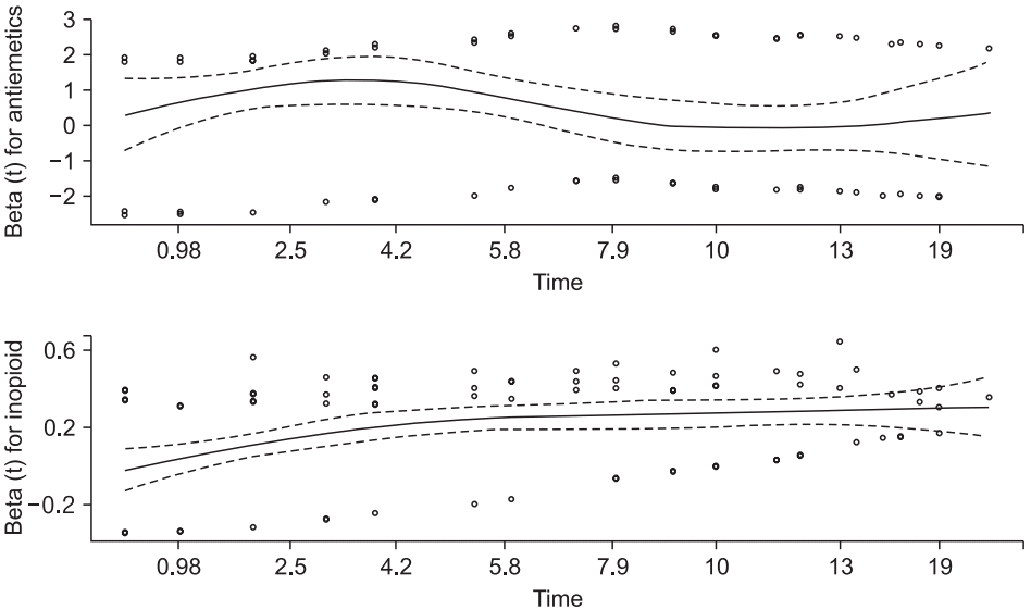
As shown in
Fig. 6, the Schoenfeld residuals of ‘Antiemetics’ and ‘Inopioid’ turn from positive to negative or vice versa at approximately 3 and 6 h. The data are arbitrarily separated using these time points.
tdc <- survSplit (Surv(Time, PONV) ~.
, data = PONV.raw
, cut=c(3, 6)
, episode = "tgroup"
, id = "id"
)
head(tdc)
The command ‘survSplit’ separates the patient data according to the established time interval, where the value for each interval is the measured value on the left side of the interval (start time, ‘tstart’), and ‘Time,’ which is the end of the interval succeeds the next interval. That is, one interval is closed at the left and opened at the right, and if an event occurs during the interval, the survival function is estimated using the variables measured at the left side of the interval (
Table 9). It seems that the data being duplicated at the end and the start of the interval, problems do not occur because the divided time does not overlap. It is possible to apply a Cox regression and GOF test with these separated data.
Table 9.
Data Divided by survSplit Function
|
No |
Antiemetics |
Age |
Wt |
Inopioid |
Survobj |
Inopioid_c |
id |
tstart |
Time |
PONV |
tgroup |
|
1 |
1 |
0 |
48 |
78.5 |
0 |
4+ |
0 |
1 |
0 |
3 |
0 |
1 |
|
2 |
1 |
0 |
48 |
78.5 |
0 |
4+ |
0 |
1 |
3 |
4 |
0 |
2 |
|
3 |
3 |
0 |
54 |
88.3 |
100 |
21+ |
1 |
2 |
0 |
3 |
0 |
1 |
|
4 |
3 |
0 |
54 |
88.3 |
100 |
21+ |
1 |
2 |
3 |
6 |
0 |
2 |
|
5 |
3 |
0 |
54 |
88.3 |
100 |
21+ |
1 |
2 |
6 |
21 |
0 |
3 |
|
︙ |
︙ |
︙ |
︙ |
︙ |
︙ |
︙ |
︙ |
︙ |
︙ |
︙ |
︙ |
︙ |
# Fitting Cox regression
fit.tdc <- coxph(Surv(tstart,Time, PONV)
~ Antiemetics:strata(tgroup)
+ Inopioid
, data = tdc)
summary(fit.tdc)
# GOF test
sf.tdc <- cox.zph(fit.tdc)
print (sf.tdc)
par(mfrow=c(2,2))
abline (h = coef(fit.tdc)[
1], lty = "dotted")
abline (h = coef(fit.tdc)[
2], lty = "dotted")
abline (h = coef(fit.tdc)[
3], lty = "dotted")
abline (h = coef(fit.tdc)[
4], lty = "dotted")
Table 10 shows the estimated Cox regression and GOF test results, and
Fig. 9 presents a plot of the Schoenfeld residuals. The risk of the PONV increases 1.0126-fold (95% CI: 1.0078–1.017, P < 0.001) by one unit of intraoperative opioid. For the antiemetics, the group taking drug B showed an increased PONV risk of 3.6545-fold (95% CI: 1.2024–11.107, P = 0.022) until 3 h post-operation, 3.8969-fold (95% CI: 1.4020–10.831, P = 0.009) until 6 h post-operation, with no significant difference shown until the end of the observation (risk ratio = 0.9382, 95% CI: 0.4242–2.075, P = 0.957). The results of the Schoenfeld residual test (
Table 10 and
Fig. 9) indicate that all variables do not violate the proportional hazard assumption. These results cannot provide a single desired outcome, and it is necessary to combine the results.
Fig. 9.
Schoenfeld residual graphs of time-dependent coefficient Cox regression.
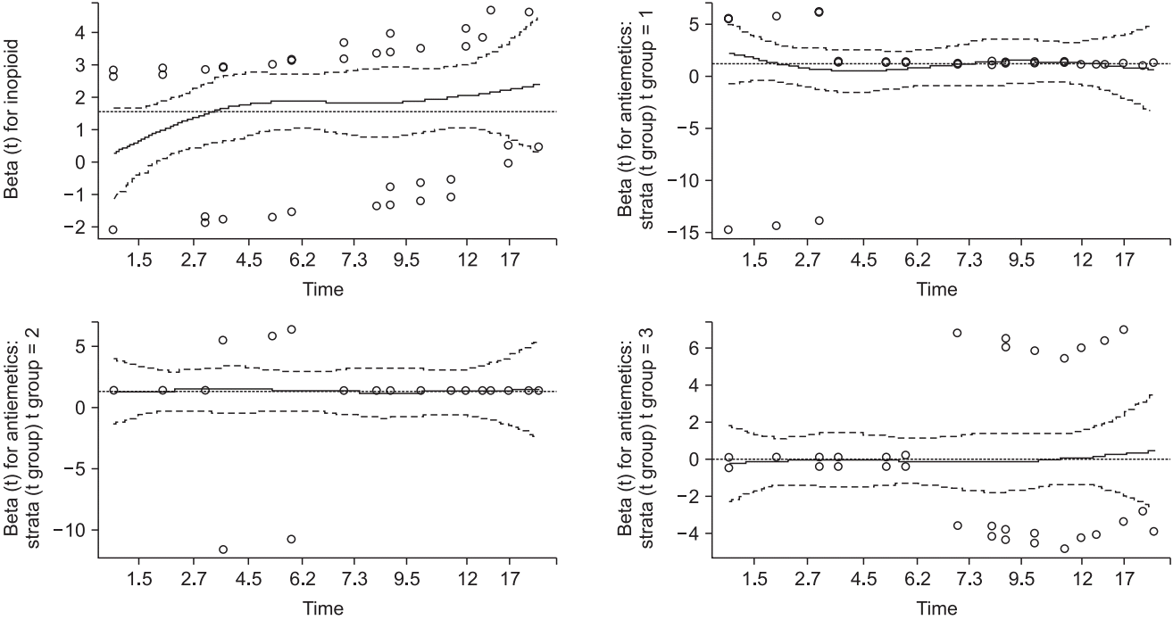
Table 10.
Results of Time-dependent Coefficient Cox Regression Using Step Function and Schoenfeld Residual Test
Call: coxph(formula = Surv(tstart, Time, PONV) ~ Antiemetics:strata(tgroup) + Inopioid, data = tdc)
|
n = 250, number of events = 63
|
|
coef |
exp(coef) |
se(coef) |
z |
Pr(>|z|) |
|
Inopioid |
0.012477 |
1.012556 |
0.002413 |
5.172 |
2.32E-07*** |
|
Antiemetics: strata(tgroup)tgroup = 1 |
1.295949 |
3.654464 |
0.567181 |
2.285 |
0.02232* |
|
Antiemetics: strata(tgroup)tgroup = 2 |
1.360185 |
3.896914 |
0.521567 |
2.608 |
0.00911** |
|
Antiemetics: strata(tgroup)tgroup = 3 |
−0.063743 |
0.938247 |
0.404993 |
−0.157 |
0.87494 |
|
--- |
|
|
|
|
|
|
Signif. codes: 0 ‘***’ 0.001 ‘**’ 0.01 ‘*’ 0.05 ‘.’ 0.1 ‘ ’ 1
|
|
exp(coef)
|
exp(-coef)
|
Lower .95
|
Upper .95
|
|
|
Inopioid |
1.0126 |
0.9876 |
1.0078 |
1.017 |
|
Antiemetics: strata(tgroup)tgroup = 1 |
3.6545 |
0.2736 |
1.2024 |
11.107 |
|
Antiemetics: strata(tgroup)tgroup = 2 |
3.8969 |
0.2566 |
1.4020 |
10.831 |
|
Antiemetics: strata(tgroup)tgroup = 3 |
0.9382 |
1.0658 |
0.4242 |
2.075 |
|
Concordance |
|
= 0.67 |
(se = 0.031) |
|
|
Rsquare |
|
= 0.152 |
(max possible = 0.874) |
|
|
Likelihood ratio test |
|
= 41.35 |
on 4 df, P = 2e-08 |
|
|
Wald test |
|
= 38.92 |
on 4 df, P = 7e-08 |
|
|
Score (logrank) test |
|
= 44.61 |
on 4 df, P = 5e-09 |
|
|
Results of Schoenfeld residual test
|
|
rho
|
chisq
|
P
|
|
|
Inopioid |
0.29948 |
5.150327 |
0.0232 |
|
Antiemetics: strata(tgroup)tgroup = 1 |
−0.02755 |
0.047411 |
0.8276 |
|
Antiemetics: strata(tgroup)tgroup = 2 |
−0.00368 |
0.000845 |
0.9768 |
|
Antiemetics: strata(tgroup)tgroup = 3 |
0.02486 |
0.038692 |
0.8441 |
|
GLOBAL |
NA |
5.199691 |
0.2674 |
# Combined results
combine.tdc <- data.frame(tstart = rep(c(0,3,6), 2)
, Time = rep(c(3,6, 24), 2)
, PONV = rep(0,12)
, tgroup= rep(1:3,4)
, trt = rep(1,12)
, prior= rep(0,12)
, Antiemetics = rep(c(0,1), each = 6)
, Inopioid = rep (c(0,1), each = 3)
, parameter = rep(0:1, each = 6)
)
combine.tdc
cfit.tdc <- survfit(fit.tdc
, newdata = combine.tdc
, id = parameter
)
cfit.tdc
km <- survfit(Surv(Time, PONV) ~Antiemetics
, data = PONV.raw
)
summary (km)
km
par( mfrow = c(1,1))
plot(km, xmax= 24, col="Black"
, lty = c("solid","dashed"), lwd=2
, xlab="Postoperative hours"
, ylab="PONV free"
)
lines(cfit.tdc, col="Grey"
, lty= c("solid","dashed"), lwd=2)
legend (x = 0.15, y = 0.25
, c("Drug A, Kaplan-Meier estimation"
, "Drug B, Kaplan-Meier estimation"
, "Drug A, Cox regression with time-dependent coefficient"
, "Drug B, Cox regression with time-dependent coefficient"
)
, col = c("black", "black", "grey", "grey")
, lty = c("solid", "dashed", "solid", "dashed")
)
To compare the results from two antiemetics, the data divided by ‘survSplit’ are combined to enable an interpretation (combine. tdc). The results are shown in
Table 11. The survival model considering the time-dependent coefficient increases the sample size because the data of one patient are separated at the established time points. Note that the median survival times in this model are 31 and 16 h, and the median survival times from the Kaplan–Meier analysis are 13 and 6 h. Plotting these two models into a single graph enables a visual comparison (
Fig. 10). Here, although ‘ggsurvplot’ provides comprehensive graphs, it cannot draw two graphs simultaneously. Another graphics software is required to make a single graph from these graphs (
Fig. 11).
Fig. 10.
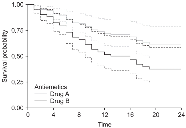
Graphical comparison between survival models of Kaplan– Meier and Cox regression with time-dependent coefficient. Black curves indicate the model fitted using a Kaplan–Meier analysis, and the gray curves are from a Cox regression with a time-dependent coefficient. The solid lines indicate Antiemetics = 0 (Drug A), and the dashed lines indicate Antiemetics = 1 (Drug B).
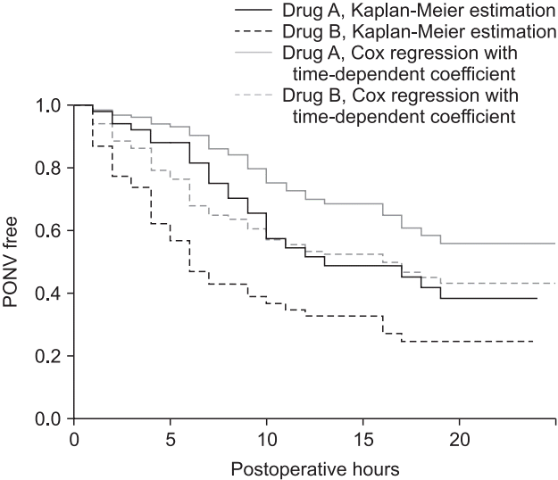
Fig. 11.
Cox regression model with the time-dependent coefficient. Survival curves of Kaplan–Meier analysis (A) and time-dependent coefficient (B) using ‘ggsurvplot’ command. Gray solid lines indicate Antiemetics = 0 (Drug A), and the black dashed lines indicate Antiemetics = 1 (Drug B). The results of the survival analysis are changed when considering the constant hazard ratio assumption.
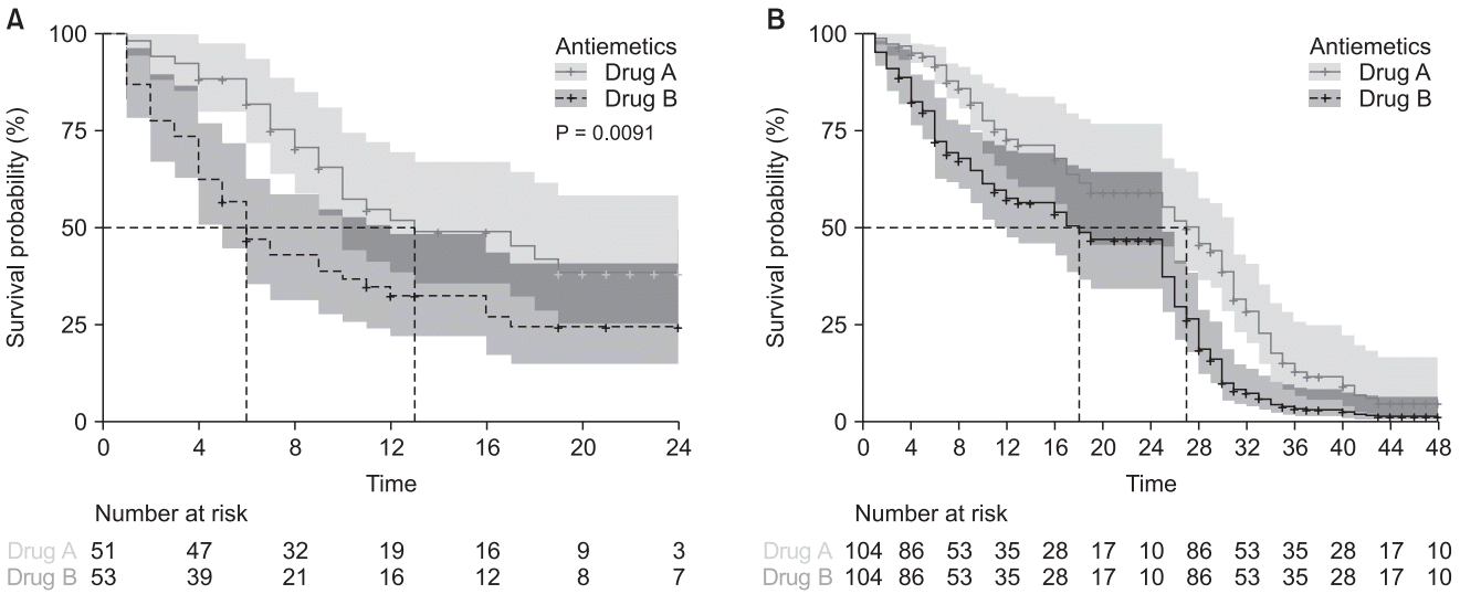
Table 11.
Comparison Kaplan–Meier Analysis and Survival Analysis with Time-dependent Coefficient
Kaplan–Meier analysis
|
|
n |
Events |
Median |
0.95LCL |
0.95UCL |
|
Antiemetics = 0 |
51 |
25 |
13 |
10 |
NA |
|
Antiemetics = 1 |
53 |
38 |
6 |
5 |
12 |
|
Survival analysis with time-dependent coefficient
|
|
n
|
Events
|
Median
|
0.95LCL
|
0.95UCL
|
|
|
0 |
104 |
126 |
31 |
17 |
40 |
|
1 |
104 |
126 |
16 |
10 |
26 |
## plot using ggsurvplot
ggsurvplot ( km, data = PONV.raw,
fun = "pct", pval = TRUE,
conf.int = TRUE, surv.median.line = "hv",
linetype = "strata", palette = "grey",
legend.title = "Antiemetics",
legend.labs = c("Drug A", "Drug B"),
legend = c(.1, .2), break.time.by = 4,
xlab = "Time (hour)",
risk.table = TRUE, tables.height = 0.2,
tables.theme = theme_cleantable(),
risk.table.y.text.col = TRUE,
risk.table.y.text = TRUE
)
ggsurvplot ( cfit.tdc, data = PONV.raw,
fun = "pct",
conf.int = TRUE, surv.median.line = "hv",
linetype = "strata", palette = "grey",
legend.title = "Antiemetics",
legend.labs = c("Drug A", "Drug B"),
legend = c(.1, .2), break.time.by = 4,
xlab = "Time (hour)",
risk.table = TRUE, tables.height = 0.2,
tables.theme = theme_cleantable(),
risk.table.y.text.col = TRUE,
risk.table.y.text = TRUE


 PDF
PDF Citation
 Print
Print


 XML Download