

 PDF
PDF Citation
 Print
Print


Introduction
Readers frequently encounter repeated measures analysis of variance (RMANOVA) when browsing the medical literature. In the field of anesthesiology, we measure blood pressure, cardiac outputs, and pain scores repeatedly at different time intervals. We can also measure blood pressure at different sites: radial and femoral, and right and left. Although RMANOVA represents a major analytical method for repeated measures (RM) data, it is frequently misused or misinterpreted due its complexity. Several articles have been published in medical journals focusing on the analysis of RM data [12]. However, despite the quality of these reports, readers of the Korean Journal of Anesthesiology (KJA), as well as potential authors, remain uncertain with regard to understanding and practically applying RMANOVA. This article focuses on three learning objectives: (1) the pitfalls of erroneously applying simple analysis of variance (ANOVA) to RM data instead of RMANOVA; (2) the obligatory sphericity assumption of RMANOVA, including adjustments and workarounds; and (3) summary measures analysis.
New readers may find it difficult to understand the statistical jargon employed in this article; therefore, several of the key technical terms and abbreviations are defined and listed presently:
· RM data is that in which two or more observations are made within an experimental unit. In the KJA, an experimental unit typically refers to a single human or animal subject. Repeated observations can occur temporally or spatially. Longitudinal data represents a special form of RM data, in which repeated observations are made over long period of time.
· RMANOVA is a distinct type of ANOVA associated with within-subject variability. Some statisticians use RMANOVA instead of univariate ANOVA to assess subject effects. In that context, RMANOVA can be considered a univariate rather than multivariate approach.
· The sum of squares (SS), which measures the variability (uncertainty, error) of data, is calculated as the sum of the squares of the distances between each observation and the mean.
- SSsomething denotes the variability explained by something known: e.g., SStime, SSgroup, and SSsubject. The total sum of squares, SStotal, is the sum of all the SS components of a dataset. If we have groups A, B, and C, then the notations can be simplified as SSA, SSB, and SSC.
- Readers should be aware that certain statistical reports use another convention, i.e., "something-SS" or "SS-something", which may be denoted as SST or TSS instead of SStotal.
· Mean squares (MS) indicates the average of the SS. MS is estimated by dividing SS by the degrees of freedom (d.f.). The ratio of each MS per MSerror is called the F value.
· Y~X denotes that "Y is modeled as X" (according to the convention of Wilkinson and Rogers, 1973) [3], which is equivalent to "Y is explained by X". When the right-hand side of the equation is empty, Y~1 equates to "Y is modeled as an interrupt," or "Y is explained by nothing," which accords with the null hypothesis.
· A : B denotes the interaction between conditions A and B.
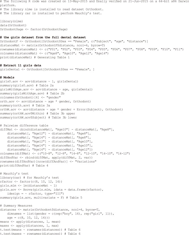
By reading this article, readers will learn typical conventions useful for interpreting full-length statistical reports; the information contained herein should act as a bridge toward understanding complex theory. All statistics were estimated using the R: A Language and Environment for Statistical Computing (ver. 3.2.0; R Foundation for Statistical Computing, Vienna, Austria). An additional library "car" (An R Companion to Applied Regression, 2nd Edition; J. Fox and S. Weisberg) was used for Mauchly's test. The complete computational procedures undertaken are attached in the appendices in R script format. The datasets introduced herein are real but have been modified slightly to aid understanding.
Go to : 
Major Differences between ANOVA and RMANOVA
A total of 16 boys and 11 girls were enrolled in a study conducted at a university dental hospital in North Carolina. Radiographic distances (mm) between the pituitary and pterygomaxillary fissure were measured repeatedly for each subject, at 8, 10, 12, and 14 years of age [4]. For simplicity, the girls' data are focused on herein, and are referred to as the "girls dataset" (Table 1).
Table 1
Dental Measurements (mm) in the "Girls Dataset" (n = 11)
The data for the 11 girls were retrieved from the full dataset (16 boys and 11 girls). originally introduced by Potthoff RF, Roy S. A generalized multivariate analysis of variance model useful especially for growth curve problems. Biometrika. 1964;51:313-26. With permission from Oxford University Press (3660581189264).
![]()
Go to :
Total Uncertainty Explained by No Factors
The initial estimation begins with a null hypothesis, e.g., "the dental measurements (in girls) were totally unexplainable," or "the dental measurements (in girls) were explained by no factors." Total SS (SST) = the SS of the error (SSE) and is computed by:
Xi,j denotes the distance on the jth occasion in the ith subject and X denotes the mean distance. SST is also computed using a simple ANOVA table that includes "nothing" as an explanatory variable (Table 2a).
Table 2
Sum of Squares for Two ANOVA Models of the "Girls Dataset" (n = 11)
![]()
Go to :
ANOVA Model of the Effect of Age
It is intuitive to hypothesize that dental distances increase with age. The effect of age can be estimated and is denoted by SSage; this approach would be incorrect unless treated as a within-subjects effect. In this model, SST is given by the sum of SSage = 50.65 and SSE = 196.7, such that SST = 247.29 of the null model (Table 2b).
Go to :
ANOVA Model of the Effects of Age, Gender, and Their Interactive Effect
Similar to the girls dataset, in the full dental measurements dataset, SST is given by the sum of SSage, SSgender, and SSage : gender (Table 3a). The models estimated thus far all exclude the effect of subject. Because the measurements for each subject were repeated four times, the SS values should have comprised SSwithin-subject and SSbetween-subject. Statistics are not correct here for effects that are repeated within-subjects, such as age and the age : gender interaction. The value of SST = 917.7 after summing all of the SS components.
Table 3
ANOVA Tables for The Full Dental Measurements Dataset (n = 27)
![]()
Go to :
RMANOVA Model of the Effects of Age, Gender, and Their Interactive Effect
We will now discuss RMANOVA (Table 3b). The ANOVA table divides sources of variability into two categories: within- and between-subjects. The effects of age (SSage = 237.19), the age : gender interaction (SSage : gender = 13.99), and its error term (SSw = 148.13) comprise the within-subject variability (SSwithin-subject). The effects of gender (SSgender = 140.5) and its error term (SSbetween = 377.9) comprise the between-subject variability (SSbetween-subject).
Perceptive readers may note that the absolute SS values equate to those of the simple ANOVA models described in the previous section; the resulting value of SST is always constant within a dataset. Changes in F values affect the calculation of P values. In the final RMANOVA model, the result of this is that the P values are either lower or higher than those listed in Table 3A, which indicates that, if RMANOVA is not used, a simple ANOVA will inflate Type I error (false-positives) in between-subject effects and Type II error (false-negative decision) in within-subject effects. A graphical approach may aid the reader in understanding the concept that total variability is comprised of several different sources of variability, denoted by the areas of the rectangles (SS; Fig. 1).
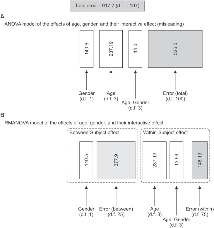 | Fig. 1Graphical representation of the concept of analysis of variance (ANOVA). The designated variabilities reduce total variability, and the areas of the rectangles denote the amount of variability. (A) ANOVA model of the effects of age, gender, and their interactive effect. (B) Repeated measures ANOVA model of the effects of age, gender, and their interactive effect. The effects of age, and the age : gender interaction, are estimated within-subjects.
|
Go to :
Sphericity Assumption
In simple terms, the variances of the differences between all combinations of measurements should be equal when using univariate RMANOVA. This is referred to as the sphericity (or circular) assumption. Sphericity, of the RM data of the covariance matrix, is strongly assumed for within-subject RMANOVA statistics. In cases that violate the sphericity assumption, within-subject RMANOVA statistics are meaningless. Given its name, i.e., "sphericity," readers may expect to encounter a relatively complicated algebraic concept, such that plain English is used to aid understanding in the discussion below.
Violations of sphericity may be evaluated using the sphericity test developed by Mauchly, which can be performed easily, or even automatically, in the majority of statistical software packages. Mauchly's test with a P > 0.05 (or 0.10 depending on your a priori assessment of the data) allows us to interpret the results of RMANOVA. Returning to the girls dataset, six pairwise differences were calculated (Table 4): 10-8, 12-8, ... , 14-12. The variances of the pairwise differences ranged from 0.60 to 1.74, which appears relatively wide; however, the Mauchly statistic (W) = 0.69, and the estimated P = 0.67, indicating that the girls dataset satisfies the sphericity assumption. A favorable result was expected for this dataset because there was no reasonable basis on which to assume the presence of another factor aside from age over the 2-year periods.
Table 4
Pairwise Differences in the "Girls Dataset" (n = 11)
![]()
To enhance the reader's understanding of the concept of sphericity, the girls dataset was modified arbitrarily by multiplying the values obtained at 12 years of age by 2. Therefore, the Mauchly statistic W = 0.15, and P = 0.006, which proves that the dataset violates the assumption. This arbitrary modification illustrates the relative rigidity of the sphericity assumption (Table 5). Because conditions between the repeated measurements should be uniform, we cannot anticipate that the assumption will be satisfied, especially when two or more conditions with brief intervals are added to a single RM dataset (e.g., administration of drugs and attempted endotracheal intubation). Such designs represent a substantial proportion of typical anesthesiology study designs.
Several "quick-and-dirty" adjustment procedures are available for RM data that violate the sphericity assumption, known as sphericity adjustments. Software packages usually provide factors (ε, epsilon) that adjust for degrees of freedom (d.f.) with respect to within-subject RMANOVA statistics. These include the Greenhouse-Geisser (ε̂) and Huynh-Feldt (ε̃) adjustment factors. By definition, the true ε values = 1, such that the sphericity assumption is fully satisfied. In the modified girls dataset described above, the Greenhouse-Geisser value ε̂ was estimated at 0.47, and the Huynh-Feldt ε̃ = 0.53. The effect of age has d.f. values of 3 (numerator) and 75 (denominator), such that the Huynh-Feldt adjusted d.f. values were as follows:
Go to :
Workarounds for RMANOVA
If the repetition has a single factor (e.g., only the time-based repetition), the calculation and interpretation of Mauchly's statistic would be easier. However, if there are more than two repetition factors, or they are nested, such calculations are rendered more difficult. Statisticians use two distinct methods to work around any violation of sphericity: multivariate analysis of variance (MANOVA) and mixed-effect modeling (MEM). Although MANOVA and MEM require more statistical knowledge, MANOVA is highly resistant to the violation of any assumption during the analysis of RM data, and MEM is a highly flexible method that uses user-defined variance structures; therefore, researchers should be familiar with both methods. We must also be aware that the editors of one international anesthesiology journal recommend MEM as the method of choice for the analysis of RM data [5]. The use of MEM should be confined to studies in which an effect of subject represents the primary concern [6].
Go to :
Summary Measure Analysis
Because the statistics-heavy results and numerous P values generated by RMANOVA often confuse researchers, they sometimes fail to notice straightforward values within their data. Everitt and Rabe-Hesketh (2001) [7], and Frison and Pocock (1992) [8], suggested that researchers should extract more direct values from RM data, such as the overall mean, maximum (minimum) value, time to maximum (minimum) response, regression slope, and time to reach a particular value. Despite a lack of consensus regarding a gold standard summary measure, after identifying data-by-data analysis becomes more straightforward, such that a t-test or simple ANOVA can be applied. In our full dental dataset, the individual mean distances and maximum distances can be calculated readily and compared between genders using a t-test (Table 6).
Go to :
 XML Download