This article has been
cited by other articles in ScienceCentral.
Abstract
Purpose
The diverse experimental environments in microarray technology, such as the different platforms or different RNA sources, can cause biases in the analysis of multiple microarrays. These systematic effects present a substantial obstacle for the analysis of microarray data, and the resulting information may be inconsistent and unreliable. Therefore, we introduced a simple integration method for combining microaray data sets that are derived from different experimental conditions, and we expected that more reliable information can be detected from the combined data set rather than from the separated data sets.
Materials and Methods
This method is based on the distributions of the gene expression ratios among the different microarray data sets and it transforms, gene by gene, the gene expression ratios into the form of the reference data set. The efficiency of the proposed integration method was evaluated using two microarray data sets, which were derived from different RNA sources, and a newly defined measure, the mixture score.
Results
The proposed integration method intermixed the two data sets that were obtained from different RNA sources, which in turn reduced the experimental bias between the two data sets, and the mixture score increased by 24.2%. A data set combined by the proposed method preserved the inter-group relationship of the separated data sets.
Conclusion
The proposed method worked well in adjusting systematic biases, including the source effect. The ability to use an effectively integrated microarray data set yields more reliable results due to the larger sample size and this also decreases the chance of false negatives.
Keywords: Microarray, Gene expression, Integration method, Different platforms, Different RNA sources, Systematic effects
INTRODUCTION
DNA microarrays are a useful tool for studying complex systems and they are being applied to many areas of the biological sciences. However, systematic biases due to different handling procedures are often present and they are a challenge in these types of experimental studies. Microarray experiments are often performed over many months and different institutions may collect and process the samples, which may be assayed by using different array hybridization protocols or by using different microarray print batches or platforms. These systematic biases can be detected as differences in the gene expression patterns when one microarray data set is compared directly with other microarray data set and, as a result, this obscures the true biological information. Hence, these systematic biases from the differences in the experimental conditions present a substantial obstacle for the analysis of microarray data.
Due to the limited number of microarray experiments that have been performed, the use of whole data sets is increasing, regardless of the platforms or the experimental procedures used. When such data sets that are derived from different experimental processes were analyzed individually, the results of the analysis were often inconsistent and they contained little reliable information. Therefore, it is necessary to investigate methods that would effectively combine microarray data sets that are derived from different experimental environments in order to minimize systematic bias.
Many studies have analyzed several independently collected microarray data sets and these studies have focused on the differential gene expressions by comparing two or more data sets in order to find the discriminative genes that can classify the different experimental groups (
1~
8). These studies have exploited the possibility of identifying more robust data sets with using multiple data sets rather than a single data set. The integration of separate data sets has the same effect of increasing the sample size of a single microarray (
9), and so this allows performing analysis of multiple microarray data sets to overcome one of the main limitations of single microarray data set, that is, a small sample size. However, a proper integration method has not yet been established and one of the previous studies suggested that microarray data sets that are derived from different experimental processes could not be combined directly because these studies have shown that there is poor correlation between the arrays (
10).
The integration of multiple data sets prior to selecting the significant gene has been recently introduced. Singular Value Decompositions (SVDs) were used to correct the systematic bias of multiple data sets, and this was used in yeast cell cycle experiments (
11) and for a data set that contained information on many soft tissue tumors (
12). SVD is a method to remove systematic effects by projecting the expression ratios onto the directions of large variation, but it has been suggested that SVD may be inappropriate to use when the magnitude of the systematic effect variation is similar to the other components of variations (
13). Meanwhile, Distance Weighted Discrimination (DWD), which is the modified form of the Support Vector Machine (SVM), and which adjusts for systematic effects, could eliminate the source effect, and it has demonstrated good performance (Benito et al., 2004). However, DWD could not regulate the dispersion of the different data sets.
A method that transforms the distributions of the gene expressions of two data sets similarly was proposed (
14). However, this method did not consider the biological differences between the two different experimental groups, such as the normal group and the tumor group because the authors used the average expression value of these two groups to define a reference sample. A recent study introduced an Analysis of Variance (ANOVA) model to select the discriminative genes from several datasets that were derived from different experimental environments (
15). This flexible method can consider any clinical variables as well as genetic information, including several effect factors that represent experimental conditions. But with this method, we can not evaluate how well the datasets are intermixed, and we can not explore the expression patterns of any interesting genes in a combined data set. Therefore, in this study, we suggest a method to effectively integrate different experimental environments.
MATERIALS AND METHODS
1) Data source
(1) Tissue sample preparation
A total of 158 colorectal tissues (84 tumors and 74 normal tissues) were obtained from colorectal cancer patients who underwent surgery at Severance Hospital in the Yonsei University College of Medicine, Seoul, Korea. Informed consent was obtained from the patients in order to use their surgical specimens and the clinicopathologic data for research purposes. The fresh tissues obtained were snap-frozen and stored at -80℃.
(2) Microarray
The total RNA was extracted from the tissues by using Trizol reagent (Invitrogen, Grand Island, NY) according to the manufacturer's protocol. The extracted RNA was purified prior to using an RNeasy kit for probe preparation (Qiagen, Germany) by following the manufacturer's protocol. The purified RNA samples were divided into two groups for gene expression profiling with using the total RNA and the amplified mRNA. Gene expression profiling on the total RNA was performed for 20 paired normal colon and tumor tissues, 23 tumor tissues and 15 normal colon tissues. The remaining 36 paired samples, 5 tumor tissues and 3 normal colon tissues were used for gene expression profiling with the amplified mRNA. The linear T7 mRNA amplification method was used for mRNA amplification with using the Megascript T7 kit (Ambion, Austin, TX) and by following the manufacturer's protocol. The total RNA (50 ug) and amplified mRNA (2 ug) were directly labelled with Cy5-dUTP and transcribed into cDNA. The microarray experiment was performed according to a reference design with the Cy-3 dUTP labeled Yonsei reference RNA. We used the 17K human cDNA microarray (GenomicTree Co., Korea) for probe hybridization based on the Yonsei CMRC protocol (
16). Following the hybridization, the microarrays were scanned using a GenePix 4000B (Axon Ins., Foster City, CA), and the images were analyzed using a GenePix Pro 4.0 (Axon Ins., Foster City, CA).
The only difference between these two microarray data sets was the source of the RNA. Previous studies have concluded that it is vital to use equally treated samples for any particular study, and all other samples should be amplified when one sample requires amplification. In addition, the sensitivity to detect differential gene expressions from the microarray data set with using amplified RNA was also different compared to using the total RNA (
17,
18). Therefore, we used these two data sets for evaluating our method.
2) Data normalization
The expression intensities were normalized so that they had similar distributions across a series of arrays. In this study, the MAD (median-absolute-deviation) scale estimator was replaced with the median-absolute-value and the A-values were normalized, as well as the M-values. Within-slide normalization transformed the expression values in order to make the intensities consistent within each array, and between-slide normalization transformed the expression values in order to achieve consistency between the arrays. Between-slide normalization was applied to the expression data because there were different dispersions between the arrays after within-slide normalization. The normalization process was executed using the 'limma' library of the R package (
http://www.r-project.org) for both within-slide and between-slide normalization.
3) Data transformation
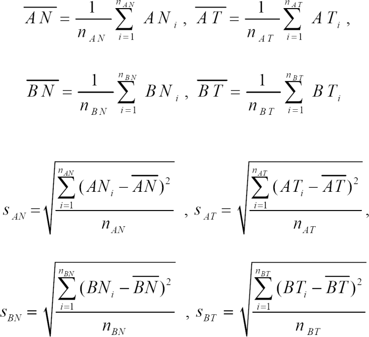
The gene expression ratios of data set A were transformed into the form of data set B when assigning data set B as the reference data set. The transformed expression ratios of the normal and tumor groups in data set A were calculated as follows for each gene.
where AN and AT are the normal and tumor groups in data set A.
AN' and AT' are the transformed expression ratios of the normal and tumor groups in data set A.
nAN, nAT are the number of experiments of the normal and tumor groups in data set A. nBN, nBT are the number of experiments of the normal and tumor groups in data set B.
4) Evaluation of data set integration
The proposed integration method was evaluated by the plots and by the newly defined metric known as the mixture score.
(1) Boxplot
A boxplot, which shows the shape of the distribution, its central value and variability, consists of the most extreme values in the data set (the maximum and minimum values), the lower and upper quartiles and the median. It is used for comparing the expression patterns of two different data sets.
(2) Dendrogram
A dendrogram is tree diagram that's frequently used to illustrate the arrangement of the clusters produced by a clustering algorithm and it is often used to illustrate the clustering of genes or experiments. It was used in order to explore whether the experiments in different data sets were well-intermixed by the proposed method. The euclidean distance was used as a similarity measure and the average linkage method was used in this work.
(3) Density plot for the gene expression distribution
The distributions of expression values of 20 randomly selected genes were observed with using a density plot to compare the different integration methods. The function 'density' in R (the R-project) was used in order to compute kernel density estimates using 'Gaussian' distribution and 512 was used as the number of equally spaced points at which the density was to be estimated.
(4) Plots for the two principal components (PC)
The PCs is a set of variables that defines a projection that encapsulates the maximum amount of variation in a data set. It is orthogonal and therefore uncorrelated to the previous principle component of the same data set. Plots for two PCs were considered for the evaluation of the proposed method.
(5) Correlation coefficient
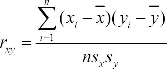
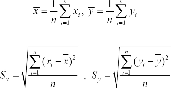
A correlation coefficient is a number between -1 and 1 that measures the degree to which two variables are linearly related and it is calculated as follows.
where x and y are two experiments.
χi is the ith gene in experiment x, and n is the number of genes in experiment x.
If there is a perfect linear relationship with a positive slope between the two variables, then we have a correlation coefficient of 1. A mean value of the correlation coefficients was used to evaluate whether the similarities of the gene expression patterns from the same experimental groups were preserved in the integrated data set by the proposed method.
(6) Mixture score
A metric, Mixture score was defined to evaluate the efficiency of the proposed integration method. The principle of this metric is to measure the ratio of the number of experiments in data set A that belong to the k-nearest neighbours (kNNs) of each experiment of data set B. The metric was calculated as follows when k is the number of nearest neighbors (NNs).
Mixture score = #{x/x∈ kNNs (data set B) ∩ (data set A)}/k
where x is any experiment belonging to kNNs (data set B) and data set A.
The mixture score ranges from 0 to 1. A value close to 0.5 means that two different data sets are perfectly intermixed and a value close to 0 or 1 means that two different data sets are not intermixed.
RESULTS
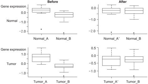
The whole data set had a range of 448 to 1,298 missing entries for each experiment, and the 12,293 genes that had no missing entries were used for further analysis. Prior to data transformation, there were significant differences in the scales and locations of the expression ratios of the randomly selected gene from the two data sets that were in the same group, as shown in
Fig. 1. However, these differences were adjusted by the transformation of the expression ratios of data set A with reference to data set B.
When we evaluated 20 randomly selected genes with using density plots, there were significant differences in the expression ratios between data set A and data set B. These differences were found in the locations of gene8 and gene13 and in the dispersions of gene6 and gene7 (
Fig. 2). If the data sets are analyzed prior to transformation, then gene6 and gene7 in data set A, which have larger variations, may be relatively more influential than those in data set B in further analysis. Due to the large differences in the locations of the expression ratios between the two different data sets, gene8 and gene13 may lose some chance to be selected as differentially expressed genes between the two experimental groups. However, after transformation of the gene expression ratios of data set A into data set B, thus preserving the expression patterns of data set A, the expression patterns of the two data sets were adjusted in further analysis.
While the two most important Principal Components (PCs) can be used in order to compare the expression patterns of two data sets, the two data sets were not only separated into the normal and tumor groups, but data set A was also separated from data set B, as shown in
Fig. 3A. This confirmed that there was a significant systematic effect in the expression ratios between the two different data sets. However, the difference in the location between the PCs from the two data sets was adjusted for by the proposed transformation method. In addition, the clear separation of the normal and tumor groups and the good mixture of the two data sets are shown with using a scatter plot (
Fig. 3B).
Unsupervised hierarchical cluster analysis was applied to the data sets in order to assess the mixture of the two data sets. Two clusters, data set A and data set B, were identified and this indicated that there was an experimental bias between the two data sets (
Fig. 4A), even though the whole gene set was able to separate the normal groups from the tumor groups within both data set A and data set B. However, in the hierarchical cluster analysis after the transformation of data set A, the transformed data set A and data set B were well intermingled, indicating that the experimental bias was minimized. Two previously identified subgroups, the normal and the tumor group, were also well separated (
Fig. 4B).
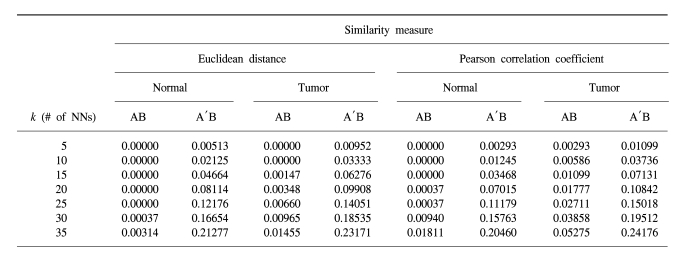
When we evaluated the mixture score of the data sets prior to transformation, the normal group within data set B was hardly intermixed with the normal group of data set A. On the other hand, the tumor group was intermixed slightly more as the number of the Nearest Neighbors (NNs) increased prior to transformation (
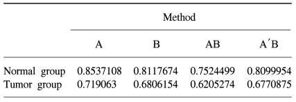
Table 1). This may be due to the larger variation within the tumor groups than that in the normal groups. The average correlation coefficient was 0.85 within the normal group in data set A, it was 0.81 in data set B, it was 0.72 within the tumor group in data set A and it was 0.68 in data set B (
Table 2). After the transformation, the
mixture scores increased by as much as 24.2% as the number of NNs were increased, suggesting that the two different data sets were well intermixed. In addition, the values were similar whether the euclidean distance or the Pearson correlation coefficient was used as a similarity measure.
The mean value of the correlation coefficients was used to evaluate how well the proposed integration method preserved the similarity of the gene expression patterns within the same groups. When the correlations within a group of an integrated data set are similar or larger than those of the individual data sets prior to integration, the proposed method can then be interpreted as having effectively integrated the data sets. Data set A had higher correlations within the same groups than did data set B prior to integration, indicating that the experiments in data set A had more homogeneous gene expression patterns than that in data set B. The integrated data set achieved by the proposed transformation method had a higher correlation coefficient within the same groups than did the combined data set prior to transformation, and this indicated that the proposed method more effectively preserved the homogeneity of the experiments within the same group.
DISCUSSION
The previous studies have encouraged the use of an integrated data set of two or more independent data sets for a variety of microarray applications (
1,
3~
9). When the microarray data sets are used without adjusting for the experimental bias and the experimental bias exceeds the biological variation, then the meaningful biological variation is not identifiable and reliable results are not obtainable. In addition, due to the limited number of microarray experiments performed, the use of whole data sets, regardless of the platforms or experimental procedures, is increasing. Therefore, adjustment of the experimental bias caused by the different experimental environments should be accounted for in further analysis of the data.
Fig. 1 showed that the expression ratios of the same genes from different data sets may be significantly different, even within the same experimental group, when microarrays from different experimental conditions are analyzed after integration without any prior transformation.
In order to minimize experimental bias in the present study, the expression ratios of a data set (data set A) were transformed to have an expression pattern that was similar to the reference data set (data set B). This transformation allowed each gene in the different data sets to have a similar expression pattern within the same experimental group. The algorithm we used was relatively simple compared to the ones used in previous studies (
11~
13). By using the proposed method, the expression patterns of genes in two data sets were transformed to have similar expression patterns, preserving the form of the distribution of the original expression ratios (
Fig. 2). From this result, we were able to confirm that the two different data sets have a fair influence on the subsequent analysis.
The double matrix of the 1D and 2D PCA (Principal Component Analysis) projections and the obvious experimental bias are shown in
Fig. 3. The diagonal plots of the first two PCs are shown as density plots. The other diagonal plots showed the relationship of a pair of two PCs as scatter plots. Two PCs were selected from two different data sets and they had similar expression patterns, but there were differences in the location of the expression ratios. However, the two different data sources were very well mixed after the transformation was performed, meaning that the systematic sample source effects in these two data sets were effectively removed. The representative expression patterns of these two data sets became similar to one another via the process of transformation, which was a problem that was not solved in a previous study (
13).
As seen in
Fig. 4A, there was no intermixture of the two data sets prior to transformation. Meanwhile, data set A and data set B were separated into normal and tumor groups within each data set with using the whole gene set. After transformation, there was a great intermixing of the two different data sets, but some of the data set in the end-node of the dendrogram had not been intermixed, as is shown in
Fig. 4B. This may have been due to the usage of a whole gene set, not a discriminative gene set, for clustering. Two previously identified subgroups, the normal and tumor subsets, separated well in the intermixed data set.
A metric measuring how well the two data sets were mixed (the
mixture score), can be interpreted that the experimental bias was removed as the value was large. The two data sets were mixed well by the proposed method, but the
mixture score was less than 25%, which is lower than the ideal perfect mixture value, suggesting that the two data sets were not yet perfectly intermingled. This may have been caused by the characteristics of the experiments included in the two data sets. The proposed method was more effective in the tumor group than in the normal group (
Table 1), which is a more heterogeneous population biologically. Therefore, the current method might be more effective in those experiments with larger variations among the experiments, as in the tumor group. In addition, on comparison of the average correlation coefficients, the tumor groups had lower correlation coefficients than did the normal groups, suggesting that the tumor groups were more heterogeneous and this may have been due to various tumor stages within the group. Consequentially, the tumor groups were intermixed better by the proposed integration method than the normal groups.
The proposed integration method transformed the expression ratios of the two data sets similarly in the corresponding experimental group, thus preserving the expression patterns of the data sets prior to transformation. Our method considered the biological differences among different experimental groups by transforming the expression ratios for each experimental group. This may distort the differences between the tumor and the normal groups and so cause false positive results, but this is a problem that may not be considered when the ranking approach is used for selection of a discriminative gene set. We used two microarray data sets that used amplified and non-amplified RNA sources for evaluating our method. Even though previous studies have concluded that equally treated samples for any particular study are essential (
18), and we also confirmed that there were clear biases between the two data sets with using unsupervised hierarchical clustering, this may not be sufficient to show that our method has general applicability. Therefore, we are currently evaluating the method with using other publicly available data sets that were experimented on with using different platforms.
When selecting the reference data set, we considered data set B as a reference data set in this work, without any consideration of the biological meaning. The data set A also can be used as a reference data set or both of two data sets can be transformed with using pooled standard deviations.
The proposed method can be used for any data set with more than two experimental groups, and it is able to combine more that 2 data sets. However, this method might not be appropriate when the different experimental features in the different data sets include biological differences (for example, early disease stages I and II in data set A and advanced disease stages III and IV in data set B). This is because the proposed method transforms the expression values of a specific experimental group into the form of a corresponding experimental group of the reference data set. Hence, we suggest using the current method for the integration of data sets, of which each data set is phenotypic or biologically homogenous, at least to the experimenters' current knowledge.
CONCLUSIONS
The proposed method worked well for adjusting systematic biases, including the source effect. The ability to use an effectively integrated microarray data set yields more reliable results due to the larger sample size and it also decreases the chance of false negatives. The discriminative gene set, which was selected from the integrated data set by our method, is expected to include more significant biological pathways.
ACKNOWLEDGMENT
We thank the members of the National Biochip Research Center, Yonsei University, and the Genomic Tree Incorporation, Korea for the current project. Special thanks goes to Tae Soo Kim for the tissue collection, Won Ju Noh for the clinical data achievement, and Chan Hee Park, Gui Youn Lee, Jae Jun Jung, Seung Hui Kang, Sun Jeong Kim and Ji Eun Kim for supporting the experiment.
References
1. Breitling R, Sharif O, Hartman ML, Krisans SK. Loss of compartmentalization causes misregulation of lysine biosynthesis in peroxisome-deficient yeast cells. Eukaryot Cell. 2002; 1:978–986. PMID:
12477798.

2. Lee PD, Sladek R, Greenwood CM, Hudson TJ. Control genes and variability: absence of ubiquitous reference transcripts in diverse mammalian expression studies. Genome Res. 2002; 12:292–297. PMID:
11827948.

3. Rhodes DR, Barrette TR, Rubin MA, Ghosh D, Chinnaitan AM. Meta-analysis of microarrays: interstudy validation of gene expression profiles reveals pathway dysregulation in prostate cancer. Cancer Res. 2002; 62:4427–4433. PMID:
12154050.
4. Choi JK, Yu U, Kim S, Yoo OJ. Combining multiple microarray studies and modeling interstudy variation. Bioinformatics. 2003; 19(Suppl 1):I84–I90. PMID:
12855442.

5. Detours V, Dumont JE, Bersini H, Menhaut C. Integration and cross-validation of high-throughput gene expression data: Comparing heterogeneous data sets. FEBS Lett. 2003; 546:98–102. PMID:
12829243.

6. Ramaswamy S, Ross KN, Lander ES, Golub TR. A molecular signature of metastasis in primary solid tumors. Nat Genet. 2003; 33:49–54. PMID:
12469122.

7. Xin W, Rhodes DR, Ingold C, Chinnaiyan AM, Rubin MA. Dysregulation of the annexin family protein family is associated with prostate cancer progression. Am J Pathol. 2003; 162:255–261. PMID:
12507908.

8. Sorlie T, Tibshirani R, Parker J, Hastie T, Marron JS, Nobel A, et al. Repeated observation of breast tumor subtypes in independent gene expression data sets. Proc Natl Acad Sci USA. 2004; 100:8418–8423. PMID:
12829800.
9. Choi JK, Choi JY, Kim DG, Choi DW, Kim BY, Lee KH, et al. Integrative analysis of multiple gene expression profiles applied to liver cancer study. FEBS Lett. 2004; 565:93–100. PMID:
15135059.
10. Kuo WP, Jenssen TK, Butte AJ, Machado LO, Kohane IS. Analysis of matched mRNA measurements from two different microarray technologies. Bioinformatics. 2002; 18:405–412. PMID:
11934739.

11. Alter O, Brown PO, Botstein D. Singular value decomposition for genome-wide expression data processing and modelling. Proc Natl Acad Sci USA. 2000; 97:10101–10106. PMID:
10963673.
12. Nielsen TO, West RB, Linn SC, Alter O, Knowling MA, O'connel J. Molecular characterisation of soft tissue tumours: a gene expression study. Lancet. 2002; 359:1301–1307. PMID:
11965276.

13. Benito M, Parker J, Du Q, Wu J, Xiang D, Perou CM, et al. Adjustment of systematic microarray data biases. Bioinformatics. 2004; 20:105–114. PMID:
14693816.

14. Jiang H, Deng Y, Chen HS, Tao L, Sha Q, Chen J, et al. Joint analysis of two microarray gene-expression data sets to select lung adenocarcinoma marker genes. BMC Bioinformatics. 2004; 5:81. PMID:
15217521.
15. Park T, Yi SG, Shin YK, Lee SY. Combining multiple microarrays in the presence of controlling variables. Bioinformatics. 2006; 2:1682–1689. PMID:
16705015.

16. Kim TM, Jeong HJ, Seo MY, Kim SC, Cho G, Park CH, et al. Determination of genes related to gastrointestinal tract origin cancer cells using a cDNA microarray. Clin Cancer Res. 2005; 11:79–86. PMID:
15671531.
17. Feldman AL, Costouros NG, Wang E, Qian M, Marincola FM, Alexander HR, et al. Advantages of mRNA amplification for microarray analysis. Biotechniques. 2002; 33:906–914. PMID:
12398200.

18. Schneider J, Buness A, Huber A, Volz J, Kioschis P, Hafner M, et al. Systematic analysis of T7 RNA polymerase based in vitro linear RNA amplification for use in microarray experiments. BMC Genomics. 2004; 5:29. PMID:
15119961.




 PDF
PDF Citation
 Print
Print




 XML Download