Journal List > Healthc Inform Res > v.27(1) > 1146459

Jang, Kim, and Yoon: Effectiveness of Transfer Learning for Deep Learning-Based Electrocardiogram Analysis

Abstract

Objectives

Many deep learning-based predictive models evaluate the waveforms of electrocardiograms (ECGs). Because deep learning-based models are data-driven, large and labeled biosignal datasets are required. Most individual researchers find it difficult to collect adequate training data. We suggest that transfer learning can be used to solve this problem and increase the effectiveness of biosignal analysis.

Methods

We applied the weights of a pretrained model to another model that performed a different task (i.e., transfer learning). We used 2,648,100 unlabeled 8.2-second-long samples of ECG II data to pretrain a convolutional autoencoder (CAE) and employed the CAE to classify 12 ECG rhythms within a dataset, which had 10,646 10-second-long 12-lead ECGs with 11 rhythm labels. We split the datasets into training and test datasets in an 8:2 ratio. To confirm that transfer learning was effective, we evaluated the performance of the classifier after the proposed transfer learning, random initialization, and two-dimensional transfer learning as the size of the training dataset was reduced. All experiments were repeated 10 times using a bootstrapping method. The CAE performance was evaluated by calculating the mean squared errors (MSEs) and that of the ECG rhythm classifier by deriving F1-scores.

Results

The MSE of the CAE was 626.583. The mean F1-scores of the classifiers after bootstrapping of 100%, 50%, and 25% of the training dataset were 0.857, 0.843, and 0.835, respectively, when the proposed transfer learning was applied and 0.843, 0.831, and 0.543, respectively, after random initialization was applied.

Conclusions

Transfer learning effectively overcomes the data shortages that can compromise ECG domain analysis by deep learning.

I. Introduction

An electrocardiogram (ECG) records cardiac activity and is commonly scheduled by cardiologists. ECGs detect arrhythmic events [1], measure heart rate variability [2], predict myocardial infarction [3], and screen for contractile dysfunction [4]. In intensive care units (ICUs), ECGs are collected in real time and used to guide treatment. ECGs can now be obtained using wearable devices, and biosignals are increasingly used to monitor health [5]. Many studies have used ECGs to this end. Most studies have used summary data, such as heartbeats/min or R peak intervals. Many studies have also subjected ECG waveform data to deep learning. Attia et al. [1] showed that deep learning of only normal sinus rhythms predicted arrhythmic events in 10,000 patients.
However, most individual researchers lack the quantity of labeled ECG waveform data required for model training. Transfer learning solves this problem [6]; pretrained neural network weights derived for a different dataset are used to fine-tune the weights for the new task. This increases model accuracy, allowing model training with fewer data [7]. Transfer learning using a small dataset has been conducted to facilitate medical image analysis [8]. However, most experiments have involved image or language analysis [9], whereas the biosignal domain has received little attention. Some studies have tried to pretrain models using labelled data from a different domain and transfer its knowledge to the target ECG domain. Van Steenkiste et al. [10] utilized transfer learning to adopt human ECG knowledge to a horse ECG model, because horse ECG data was difficult to collect. Some studies have tried to adopt image domain knowledge in the ECG domain using transfer learning and have achieved good performance [1113]. Because a pretrained model was trained to classify the ImageNet dataset, which was totally different from the ECG domain, these studies had to convert one-dimensional (1D) signal to two-dimensional (2D) images. If there is a pretrained model for the ECG domain, a 2D transformation process may not be needed, and there is a possibility that the performance will be improved.
Even when using transfer learning, researchers may lack adequate labeled data for a pretraining model. Thus, many studies have sought to apply the unsupervised learning of unlabeled data to transfer learning. A model is pretrained using unlabeled big data, and the weights are then employed to solve a new problem associated with only a small labeled dataset. An autoencoder engages in unsupervised transfer learning. Wen et al. [14] classified faults using a sparse autoencoder that employs transfer learning. Wang et al. [15] developed an automated chest-screening model using transfer learning and a convolutional, sparse denoising autoencoder. Eduardo et al. [16] utilized an autoencoder and transfer learning to develop an individual identification model.
In this work, we explored whether transfer learning facilitates biosignal analysis and the influence of the biosignal datasets. We hypothesized that transfer learning would enhance model performance and reliability. We gradually reduced the size of the labeled datasets when examining the utility of transfer learning in a data-starved environment. We trained a convolutional autoencoder (CAE) using an unlabeled ECG database of Ajou University Medical Center (AUMC) [17] and re-used the CAE weights to classify 11 ECG rhythms of a dataset from a Shaoxing Hospital [18]. Transfer learning rendered the model robust, particularly when the labeled dataset was small. This is the first study to utilize unlabeled ICU ECG big data from over 25,000 patients for transfer learning in biosignal analysis and to make a pretrained ECG model and its weights available to the public.

II. Methods

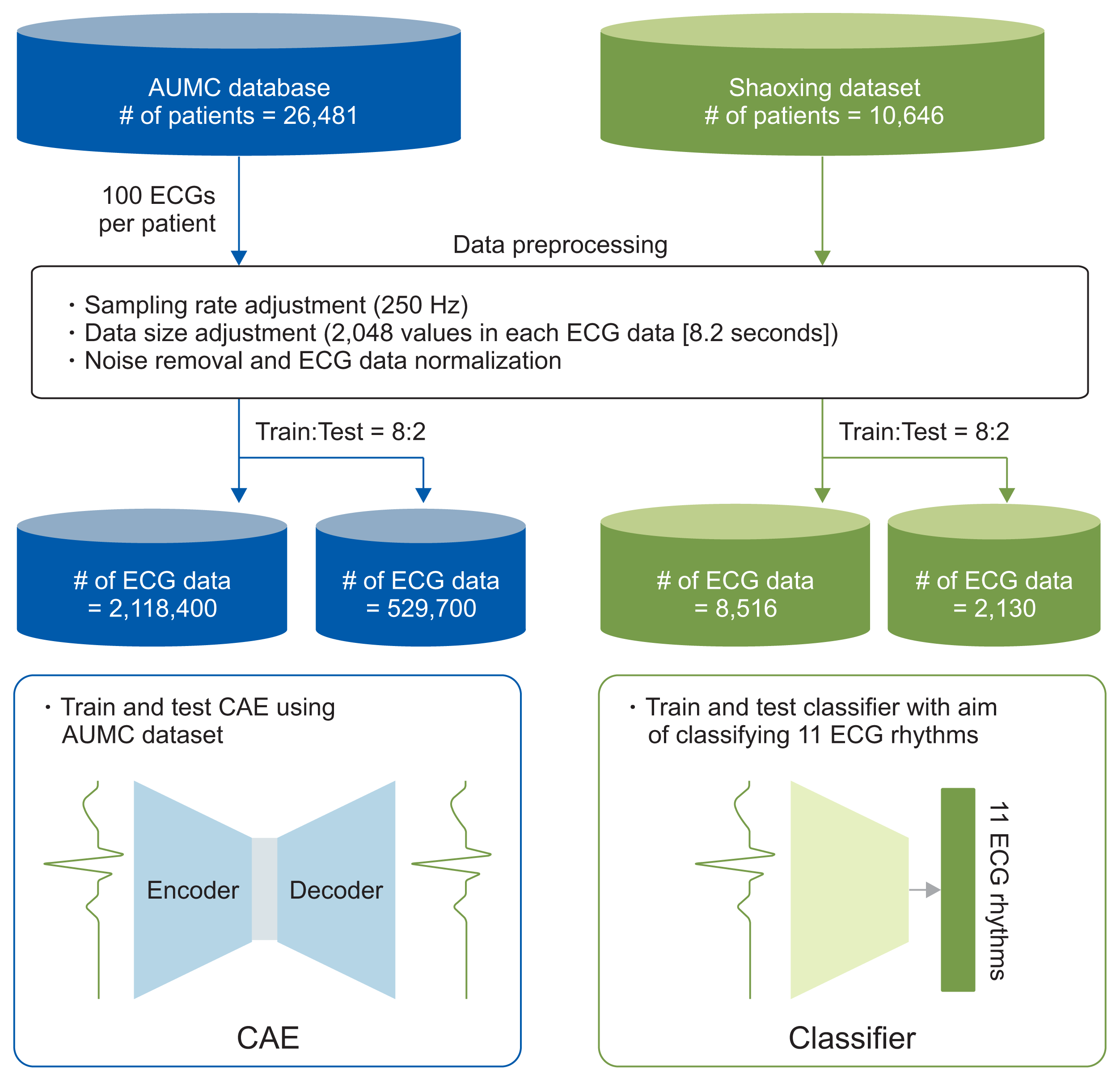
The study was approved by the Ajou University Hospital Institutional Review Board (No. YYIRB-DEV-MDB-18-497). The requirement for informed consent was waived given the retrospective nature of the work. The study proceeded in three phases (Figure 1). First, we collected two ECG datasets (a raw-waveform unlabeled database from the AUMC ICU and a 12-lead ECG dataset from the Shaoxing People’s Hospital of China) labeled in terms of 11 ECG rhythms by two physicians. We then trained the CAE using the AUMC ICU dataset, as described below. Subsequently, we classified the 11 ECG rhythms using the Shaoxing dataset. When training the classifier, we re-used the earlier weights (i.e., transfer learning) and also conducted random weight initialization; then the results were compared.

1. Data Sources

We used two ECG datasets. The AUMC ICU biosignal database was established on September 1, 2016, and it contains information on 26,481 South Korean patients (to May 10, 2020); the Shaoxing dataset contains 12-lead ECG information on 10,646 patients of the Shaoxing People’s Hospital of China. The AUMC ICU monitored patients using Nihon Kohden and Philips devices. One device yields numerical data (heartbeats/min, mean blood pressure/min, and respiratory rate/min), and the other device produces waveform data including ECGs, photoplethysmograms, and arterial blood pressure readings.
We randomly extracted 100 samples of 8.2-second-long ECG lead II data for each patient. We used a total of 2,648,100 ECG data samples and divided them into training and test datasets in an 8:2 ratio. The Shaoxing dataset consists of 10-second-long 12-lead ECGs collected using the MUSE system of GE Healthcare. All samples were labeled by a licensed physician, and another licensed physician validated the labels. Only the 10-second-long ECG lead II data were used for classification, with or without transfer learning. The Shaoxing dataset includes 11 types of ECG rhythms (normal sinus rhythms, sinus irregularities, sinus bradycardias, sinus tachycardias, supraventricular tachycardias, atrial tachycardias, sinus atrium-to-atrial wandering rhythms, atrioventricular node re-entrant tachycardias, atrioventricular re-entrant tachycardias, atrial fibrillations, and atrial flutters).

2. Data Preprocessing

To form the AUMC biosignal dataset, ECGs were collected at 250 Hz by the Nihon Kohden monitors and at 500 Hz by the Philips devices. The Shaoxing ECG data were collected at 500 Hz. To standardize the sampling rate to 250 Hz, the 500-Hz ECG data were downsampled to 250 Hz. Baseline wandering noise was removed via Butterworth filtering. We used 8.2-second-long ECG data samples to ensure that each recording featured 2,048 data points.

3. Model Development

1) Convolutional autoencoder

An autoencoder (AE) [19,20] engages in unsupervised deep learning when extracting features. An AE features an encoder and a decoder. The encoder is trained to extract ECG features into small vectors, and the decoder is trained to convert the vectors into outputs close to the original ECG data. It is assumed that the decoder outputs resemble the original data; an optimal encoder extracts ECG features well. An AE seeks to reduce the reconstruction error between the original ECG data and the reconstructed output. The mean squared error (MSE) of reconstruction was calculated. A CAE has a similar architecture, but both the encoder and decoder are convolutional neural networks (CNNs) [21]. Because ECG data are one-dimensional, the CNNs of a CAE are also one-dimensional.
Z=Encoder(X)X=Decoder(Z)MSE=i2048(Xi-Xi)2
where
  • X: original ECG data;

  • Z: feature vector;

  • X′: reconstructed ECG data;

  • Xi: the ith value of an original ECG datum (X);

  • X′i: the ith value of the reconstructed ECG datum (X′).

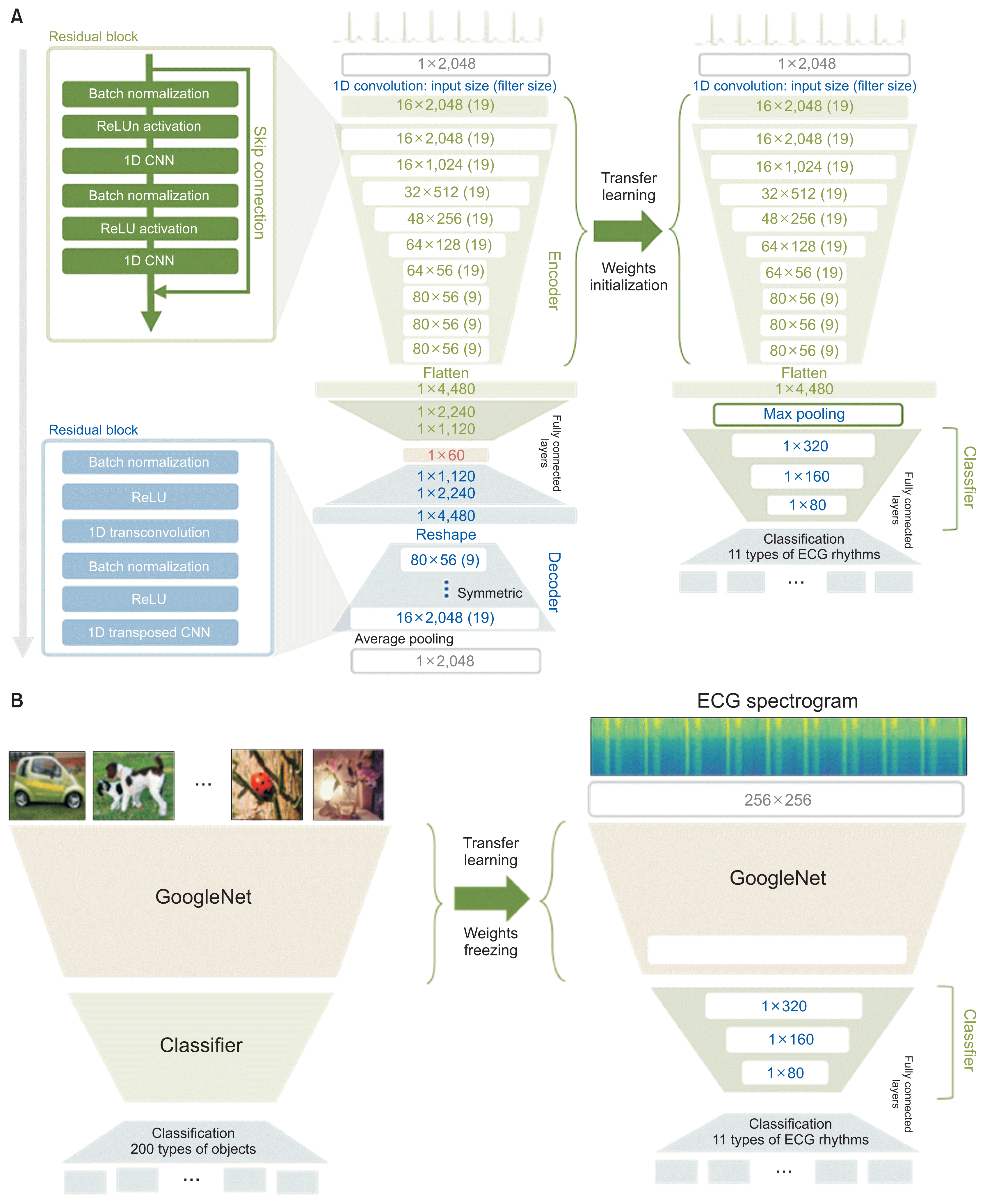
Our encoder consists of nine residual blocks containing two CNN layers, a ReLU (Rectified Linear Unit) activation function, and two batch normalization layers. The CNN layer filter sizes and strides were 19 and 1, respectively. The number of encoder-extracted features was set to 60. The decoder was of the same structure but used transposed rather than simple CNN layers (Figure 2A).

2) Proposed transfer learning strategy

Transfer learning applies the weights of a pretrained model to a model that is to perform a different task. We first trained the CAE using ECG data from the AUMC biosignal dataset. Then, we classified the ECG rhythms and compared the performance of a classifier with weighting initialization using the CAE encoder (transfer learning) and a classifier with random weight initialization (no transfer learning) (Figure 2A). During classifier training, the number of training epochs, the learning rate, the training dataset, and the optimizer were all identical; only the weighting initialization differed.

3) Comparison with another transfer learning strategy

To show that our approach is an effective transfer learning strategy using a model that has been pretrained with big data of ICU biosignal ECGs, we compared the classification performance of our approach and another approach that was suggested in previous works [1416]. They converted 1D ECG data into 2D image data as spectrograms and tried to analyze them in the 2D image domain. They utilized a model that was pretrained using an ImageNet dataset containing 4 million images for 200 categories [22], as a feature extractor. As in that previous work, we converted all ECG data in the Shaoxing dataset into 2D spectrogram images and used pretrained GoogleNet [23], which was fixed and utilized as a feature extractor. The classifier was trained and finetuned using features from the pretrained GoogleNet (Figure 2B). All experiment settings and hyperparameters were identical with our approach.

4. Evaluation

1) Evaluation of the CAE

The CAE performance was evaluated by calculating the mean reconstruction errors; smaller values indicated better performance. During AE training, the model performance was evaluated using a test dataset during each epoch, and training was stopped early when no performance improvement was evident.

2) Evaluation of ECG rhythm classification

ECG rhythm classifications were evaluated according to the weighted F1-score. Each classification task was repeated 10 times using a bootstrapping method. The results are presented as means with standard deviations [24]. The classifier was trained for 150 epochs. We employed the ADAM optimizer [25], and the learning rate was 0.005. Welch’s t-test confirmed that the two results differed (p < 0.05).
Accuracy=(TruePositive+TrueNegative)/(Totalnumberofdata)Precision=(TruePositive)/(TruePositive+FalsePositive)Recall=(TruePositive)/(TruePositive+FalseNegative)f1-score=2*(Precision*Recall)/(Precision+Recall)Weightedf1-score=i=1kwi*f1-scorei
where
  • i: index of class;

  • wi: the proportion of the class among all classes;

  • k: the number of classes.

3) Evaluation of learning curves

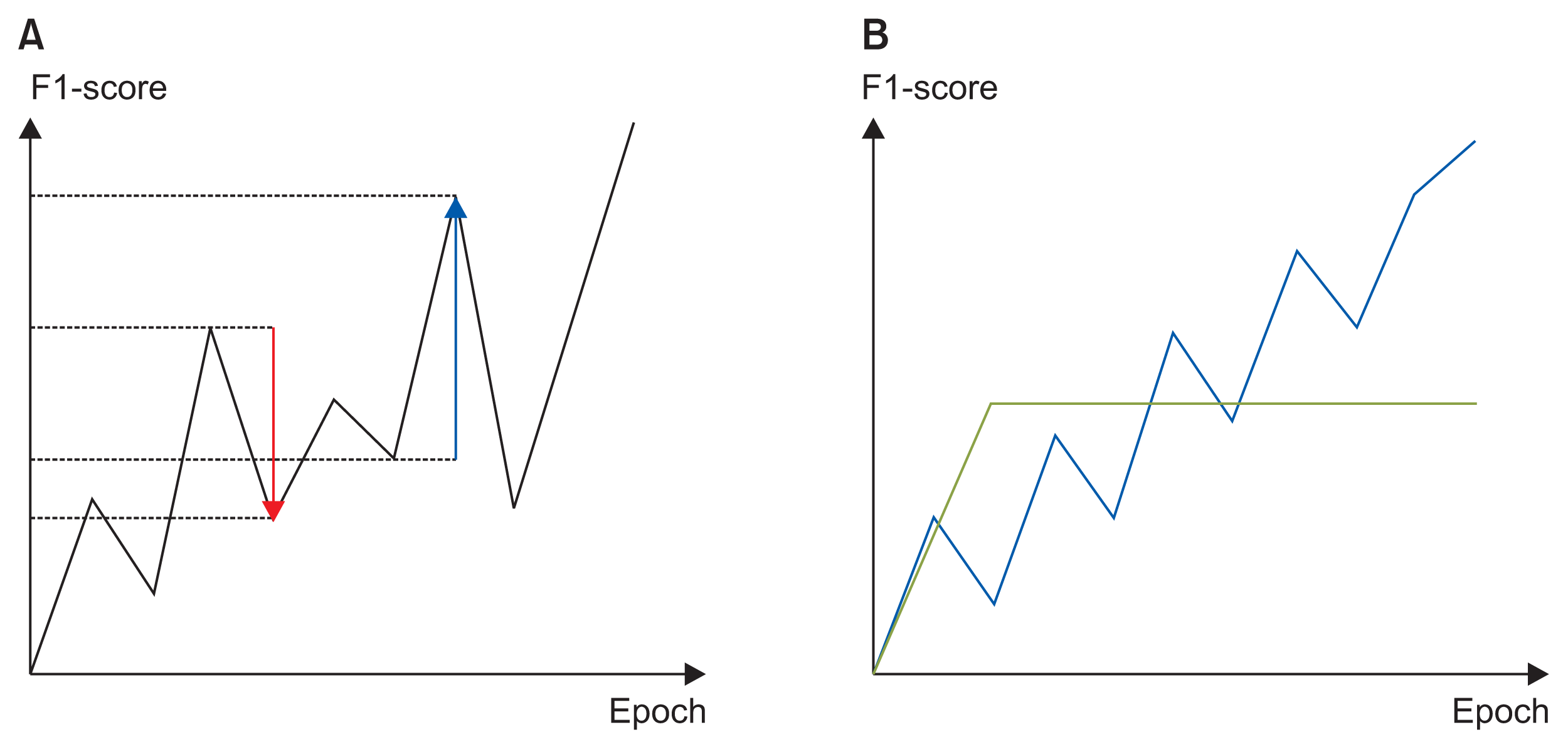
We believed that a good learning curve would exhibit continuous performance improvements, and that a high performance metric would be ultimately attained. We thus defined a new metric that we termed the learning curve index (LCI):
LCI=(meanposmeanneg+ɛ)*bestf1-score
where
  • pos: positive change in the F1-score of the test dataset for each epoch;

  • neg: negative change in the F1-score of the test dataset for each epoch;

  • ɛ: the smallest value for avoiding infinity when the mean negative value is zero.

Because the learning curve increased steadily without decreasing, the LCI became larger. In Figure 3B, the blue learning curve was better than the green learning curve. To ensure that the green curve scored lower, the best F1-scores obtained during training were multiplied.

4) Data starvation

To confirm that transfer learning became more effective as the dataset size was reduced, we compared the performance of models based on transfer learning or random initialization. We created training and test datasets in an 8:2 ratio, and used 100%, 50%, and 25% of the training dataset for training; we then employed the test dataset to evaluate performance. All tests were repeated 10 times (bootstrapping).

III. Results

We included 2,648,100 ECG data points from the AUMC biosignal database and 10,646 data points from the Shaoxing dataset. The baseline dataset characteristics are summarized in Table 1.
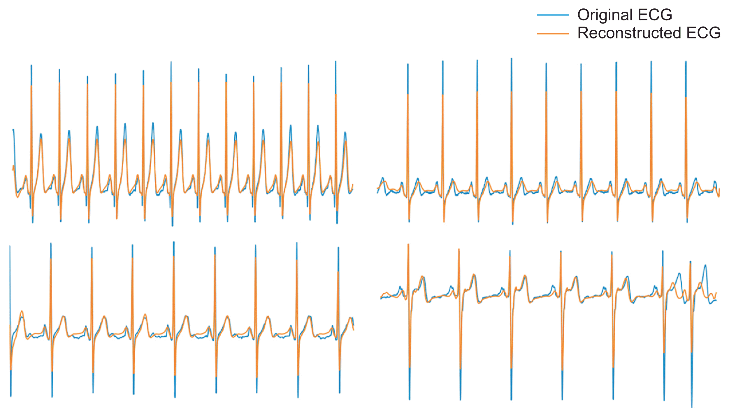
The trained CAE effectively encoded 60 features of raw ECG waveform data and decoded them to ECG waveforms (Figure 4). The mean reconstruction error was 626.583 for the AUMC test dataset. The mean error for each datum was 0.305 (626.583/2,048). Each datum featured a mean error of 3.33% when it was considered that the zero-normalized ECG data exhibited an average y-axis range of −3 to 6.
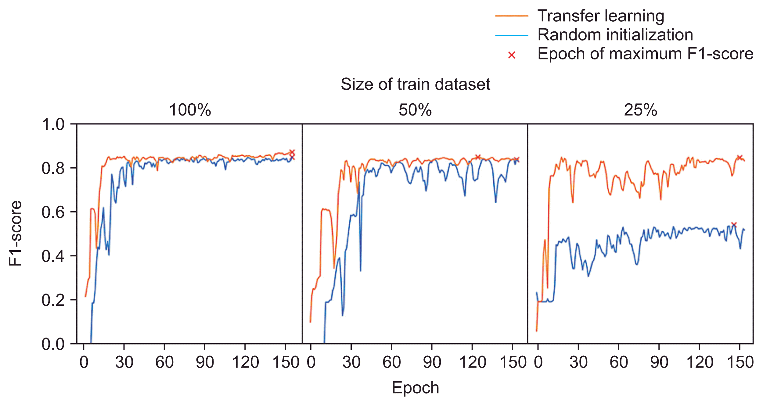
We compared the classification performance for the Shaoxing dataset when weights were randomly initialized (no transfer learning), when the CAE weights were used (proposed transfer learning in our study), and when the 2D image transfer learning approach suggested in previous works was used. The best F1-scores of the test dataset over 150 training epochs in the 10 bootstrap trials as the training dataset size was reduced from 100% to 50% and 25% are listed in Table 2. Even when all available data were used, the average F1-score associated with transfer learning was significantly higher than that associated with both random initialization and 2D transfer learning (p < 0.05). That difference became more marked as the training data numbers were reduced. When only 25% of the data were used, the performance of the random initialization model fell markedly from 0.843 to 0.543, but the F1-scores of 2D transfer learning and the proposed transfer learning remained robust at 0.782 and 0.835, respectively. However, the F1-score of the proposed transfer learning was significantly better in all case than those of the other two strategies.
When the LCI was used to evaluate learning stabilization, transfer learning provided significantly better stability when 50% or 25% of the data were used compared to random initialization (p < 0.05) (Table 3). In particular, when only 25% of the training data were used, the LCI indicated that random initialization resulted in worse performance. The LCIs were less than 1, indicating that sudden performance drops were more frequent than after complete training. By contrast, even when only 25% of the training data was used (Figure 5), the LCIs remained over 1 in most bootstrap trials featuring transfer learning.

IV. Discussion

We confirmed that the weights extracted by the CAE using ICU biosignal big data could be employed for transfer learning. The CAE reconstructed original ECG waveforms using only 60 training features. The weights employed to extract these features improved the ECG performance by stabilizing training via transfer learning, especially when the training data were sparse. The transfer learning effect was then maximal. When data are sparse, extreme values may significantly influence modeling because there is a risk that biased data will be employed. These may optimize the detection of local minima rather than the global minimum. We kept such concerns in mind during training. Figure 5 shows that sudden performance drops were more common after random initialization, and the final performance was poor when only 25% of the data were employed. The performance after final training remained poorer than that after transfer learning even when the entire dataset was used.
We compared the performance of our transfer learning approach with that of the 2D image transfer learning approach. When the proposed transfer learning pretrained an unsupervised model using unlabeled ICU ECG data, it achieved better classification performance than 2D image transfer learning. This implies that transfer learning with an unsupervised model using data from a similar domain or the same domain is more effective than transfer learning using a model pretrained with 2D domain data. When 100% or 50% of the training dataset was used, 2D image transfer learning achieved lower performance than random initialization. When only 25% of the training dataset was used, 2D transfer learning outperformed random initialization. However, in all cases, our proposed transfer learning outperformed other approaches. Because we utilize pretrained CAE weights which we are making to the public, individual researchers who need to apply transfer learning to their ECG analysis can improve the performance of their models and take advantage of having a large ECG dataset.
Thus, researchers who lack large ECG datasets can nonetheless develop diverse, robust deep-learning models. Transfer learning has been widely used in image analysis [26]. The fundamental features of general images are useful in the analysis of different images or in vision research [27]. ECG data can be used to evaluate not only the cardiovascular system but also general health or diabetes mellitus status [28]. Our research will aid the development of healthcare solutions by rendering it possible to gather large amounts of ECG data. We have placed the weights of our trained CAE model on our GitHub page (https://github.com/CMI-Laboratory/CAE).
Our work had certain limitations. We used ECG data from only one South Korean institute for CAE model training. However, we confirmed that the CAE weights were useful to train external ECG data (the Shaoxing dataset). Thus, the trained weights were not overfitted and included valuable ECG features shared by non-Korean populations, at least in Asia. The generalizability of our model to Westerners should be studied in the future. Second, our CAE model may be able to extract patterns from only short (8.2 seconds) ECG waveforms. However, long-term patterns (such as heart rate variability) are also clinically important. The extraction of long-term patterns hidden in ECG waveforms is required. Although there are more types of ECG waveforms, such as ventricular arrhythmia, we used 11 types of arrhythmia ECGs in the Shaoxing dataset to validate the ECG features from our model. However, we expect that, because the feature extraction model learned over 2 million of ECG data that naturally occurred in the ICU, more various types of ECGs could be implied in features (Supplementary Figure S1). In future research, we will validate features with more diverse types of ECGs.
In conclusion, we used a CAE to extract ECG features and showed that the CAE achieved efficient ECG classification after transfer learning. The weights of the pre-trained CAE increased model performance and stabilized training. Our results will facilitate the development of ECG-related, healthcare artificial intelligence systems.

Supplementary Materials

Supplementary materials can be found via https://doi.org/10.4258/hir.2021.27.1.19.

Acknowledgments

This work was supported by the Korea Medical Device Development Fund grant funded by the Korea government (Ministry of Science and ICT, Ministry of Trade, Industry and Energy, Ministry of Health & Welfare, and Ministry of Food and Drug Safety) (No. 202012B04). This work was also supported by grants from the Korea Health Technology R&D Project through the Korea Health Industry Development Institute (KHIDI) funded by the Ministry of Health & Welfare, Republic of Korea (Government-wide R&D Fund Project for Infectious Disease Research [GFID]; No. HG18C0067). This research was funded by the Bio Industrial Strategic Technology Development Program (No. 20001234) funded By the Ministry of Trade, Industry & Energy (MOTIE, Korea).

Notes

Conflict of Interest

No potential conflict of interest relevant to this article was reported.

Supplementary Materials

Supplementary materials can be found via https://doi.org/10.4258/hir.2021.27.1.19.

References

1. Attia ZI, Noseworthy PA, Lopez-Jimenez F, Asirvatham SJ, Deshmukh AJ, Gersh BJ, et al. An artificial intelligence-enabled ECG algorithm for the identification of patients with atrial fibrillation during sinus rhythm: a retrospective analysis of outcome prediction. Lancet. 2019; 394:861–7.
crossref
2. van Ravenswaaij-Arts CM, Kollee LA, Hopman JC, Stoelinga GB, van Geijn HP. Heart rate variability. Ann Intern Med. 1993; 118:436–47.
crossref pmid
3. Al-Zaiti S, Besomi L, Bouzid Z, Faramand Z, Frisch S, Martin-Gill C, et al. Machine learning-based prediction of acute coronary syndrome using only the pre-hospital 12-lead electrocardiogram. Nat Commun. 2020; 11:3966.
crossref pmid pmc
4. Attia ZI, Kapa S, Lopez-Jimenez F, McKie PM, Ladewig DJ, Satam G, et al. Screening for cardiac contractile dysfunction using an artificial intelligence-enabled electrocardiogram. Nat Med. 2019; 25:70–4.
crossref pmid
5. Isakadze N, Martin SS. How useful is the smartwatch ECG? Trends Cardiovasc Med. 2020; 30:442–8.
crossref pmid
6. Pan SJ, Yang Q. A survey on transfer learning. IEEE Trans Knowl Data Eng. 2009; 22:1345–59.
crossref
7. Zhao W. Research on the deep learning of the small sample data based on transfer learning. AIP Conf Proc. 2017; 1864:020018.
crossref
8. Raghu M, Zhang C, Kleinberg J, Bengio S. Transfusion: understanding transfer learning for medical imaging [Internet]. Ithaca (NY): arXiv.org;2019. [cited at 2021 Jan 4]. Available from: https://arxiv.org/abs/1902.07208.
9. Ranti D, Hanss K, Zhao S, Arvind V, Titano J, Costa A, et al. The utility of general domain transfer learning for medical language tasks [Internet]. Ithaca (NY): arXiv.org;2020. [cited at 2021 Jan 4]. Available from: https://arxiv.org/abs/2002.06670.
10. Van Steenkiste G, van Loon G, Crevecoeur G. Transfer learning in ECG classification from human to horse using a novel parallel neural network architecture. Sci Rep. 2020; 10:186.
crossref pmid pmc
11. Tadesse GA, Zhu T, Liu Y, Zhou Y, Chen J, Tian M, et al. Cardiovascular disease diagnosis using cross-domain transfer learning. Annu Int Conf IEEE Eng Med Biol Soc. 2019; 2019:4262–5.
crossref
12. Salem M, Taheri S, Yuan JS. ECG arrhythmia classification using transfer learning from 2-dimensional deep CNN features. In : Proceedings of 2018 IEEE Biomedical Circuits and Systems Conference (BioCAS); 2018 Oct 17–19; Cleveland, OH.
crossref
13. Abdelazez M, Rajan S, Chan AD. Transfer learning for detection of atrial fibrillation in deterministic compressive sensed ECG. Annu Int Conf IEEE Eng Med Biol Soc. 2020; 2020:5398–401.
crossref
14. Wen L, Gao L, Li X. A new deep transfer learning based on sparse auto-encoder for fault diagnosis. IEEE Trans Syst Man Cybern Syst. 2017; 49:136–44.
crossref
15. Wang C, Elazab A, Jia F, Wu J, Hu Q. Automated chest screening based on a hybrid model of transfer learning and convolutional sparse denoising autoencoder. Biomed Eng Online. 2018; 17:63.
crossref pmid pmc
16. Eduardo A, Aidos H, Fred A. ECG-based biometrics using a deep autoencoder for feature learning-an empirical study on transferability. In : Proceedings of the 6th International Conference on Pattern Recognition Applications and Methods; 2017 Feb 24–26; Porto, Portugal. p. 463–70.
crossref
17. Yoon D, Lee S, Kim TY, Ko J, Chung WY, Park RW. System for collecting biosignal data from multiple patient monitoring systems. Healthc Inform Res. 2017; 23:333–7.
crossref
18. Zheng J, Zhang J, Danioko S, Yao H, Guo H, Rakovski C. A 12-lead electrocardiogram database for arrhythmia research covering more than 10,000 patients. Sci Data. 2020; 7:48.
crossref pmid pmc
19. Baldi P. Autoencoders, unsupervised learning, and deep architectures. In : Proceedings of the International Conference on Machine Learning (ICML): Unsupervised and Transfer Learning; 2012 Jun 26–Jul 1; Edinburgh, Scotland. p. 37–49.
20. Liu W, Wang Z, Liu X, Zeng N, Liu Y, Alsaadi FE. A survey of deep neural network architectures and their applications. Neurocomputing. 2017; 234:11–26.
crossref
21. Qin Z, Yu F, Liu C, Chen X. How convolutional neural network see the world-A survey of convolutional neural network visualization methods [Internet]. Ithaca (NY): arXiv.org;2018. [cited at 2021 Jan 4]. Available from: https://arxiv.org/abs/1804.11191.
22. Deng J, Dong W, Socher R, Li LJ, Li K, Li FF. ImageNet: a large-scale hierarchical image database. In : Proceedings of 2009 IEEE Conference on Computer Vision and Pattern Recognition; 2009 Jun 20–25; Miami, FL. p. 248–55.
crossref
23. Szegedy C, Liu W, Jia Y, Sermanet P, Reed S, Anguelov D, et al. Going deeper with convolutions. In : Proceedings of the IEEE Conference on Computer Vision and Pattern Recognition; 2015 Jun 7–12; Boston, MA. p. 1–9.
crossref
24. DiCiccio TJ, Efron B. Bootstrap confidence intervals. Stat Sci. 1996; 11:189–212.
crossref
25. Kingma DP, Ba J. Adam: a method for stochastic optimization [Internet]. Ithaca (NY): arXiv.org;2014. [cited at 2021 Jan 4]. Available from: https://arxiv.org/abs/1412.6980.
26. Hussain M, Bird JJ, Faria DR. A study on CNN transfer learning for image classification. Lotfi A, Bouchachia H, Gegov A, Langensiepen C, McGinnity M, editors. Advances in computational intelligence systems. Cham, Switzerland: Springer;2018. p. 191–202.
crossref
27. Huh M, Agrawal P, Efros AA. What makes ImageNet good for transfer learning? [Internet]. Ithaca (NY): arXiv. org;2016. [cited at 2021 Jan 4]. Available from: https://arxiv.org/abs/1608.08614.
28. Porumb M, Stranges S, Pescape A, Pecchia L. Precision medicine and artificial intelligence: a pilot study on deep learning for hypoglycemic events detection based on ECG. Sci Rep. 2020; 10:170.
crossref pmid pmc

Figure 1
Overview of the study. Two electrocardiogram (ECG) dataset were used for this study. In the preprocessing stage, ECG data from two dataset were adjusted for transfer learning. Ajou University Medical Center (AUMC) ECG data were used for training of the convolutional autoencoder (CAE) model. Shaoxing Hospital ECG data were used for training the classification model with 11 types of ECGs.
hir-27-1-19f1.gif
Figure 2
Structure of the convolutional autoencoder (CAE) and that of two transfer learning strategies. (A) The CAE was pre-trained using the Ajou University Medical Center (AUMC) ECG dataset, and the CAE weights were employed for transfer learning to initialize the ECG rhythm classifier. (B) Structure of a two-dimensional transfer learning strategy suggested in a previous work. It utilized GoogleNet pretrained with an ImageNet dataset. ECG: electrocardiogram.
hir-27-1-19f2.gif
Figure 3
Examples of learning curves and LCIs. (A) Red and blue arrows indicate negative and positive changes, respectively. (B) Two sample learning curves; the blue curve indicates better learning performance than the green curve. LCI: learning curve index.
hir-27-1-19f3.gif
Figure 4
Examples of electrocardiogram (ECG) reconstructed by the convolutional autoencoder (CAE). The latter are similar to the original ECGs. The CAE reliably extracted and reconstructed variously shaped ECG data.
hir-27-1-19f4.gif
Figure 5
Examples of learning curves for each data-starvation experiment. When 100% of the training dataset was used, the two learning curves did not appear to differ. When less than 50% of training dataset was used, the learning curves became unstable. However, the learning curves associated with transfer learning seemed more stable and indicated better performance than the learning curves associated with random initialization.
hir-27-1-19f5.gif
Table 1
Baseline characteristics of patients in both datasets
Characteristic AUMC dataset (n = 26,481) Shaoxing dataset (n = 10,646)
Age (yr) 61.056 ± 20.172 59.2 ± 18.002
Sex, male 16,370 (61.817) 5,956 (55.946)
ECG data count 2,648,100 10,646
ECGs per patient 100 1

Values are presented as mean ± standard deviation or number (%).

AUMC: Ajou University Medical Center, ECG: electrocardiogram.

Table 2
Best F1-scores of the test dataset for all bootstrapping trials
Trial # Size = 100% Size = 50% Size = 25%


Random initialization Image transfer Transfer learning Random initialization Image transfer Transfer learning Random initialization Image transfer Transfer learning
1 0.838 0.812 0.861 0.833 0.797 0.849 0.546 0.781 0.832

2 0.850 0.812 0.853 0.835 0.801 0.836 0.537 0.784 0.838

3 0.843 0.806 0.863 0.839 0.797 0.844 0.554 0.781 0.844

4 0.844 0.808 0.861 0.826 0.795 0.845 0.551 0.779 0.832

5 0.843 0.821 0.849 0.825 0.798 0.845 0.549 0.784 0.837

6 0.852 0.812 0.855 0.831 0.800 0.842 0.54 0.781 0.839

7 0.841 0.814 0.854 0.834 0.797 0.842 0.529 0.787 0.815

8 0.843 0.813 0.856 0.833 0.791 0.845 0.541 0.779 0.836

9 0.839 0.814 0.859 0.824 0.794 0.84 0.533 0.780 0.832

10 0.843 0.800 0.859 0.833 0.791 0.841 0.552 0.781 0.845

Mean ± SD 0.843 ± 0.004 0.811 ± 0.005 0.857 ± 0.004 0.831 ± 0.005 0.796 ± 0.003 0.843 ± 0.004 0.543 ± 0.009 0.782 ± 0.003 0.835 ± 0.008

p-value <0.05 <0.05 <0.05

Image transfer: transfer learning using spectrogram via pretrained model with ImageNet dataset, Transfer learning: proposed transfer learning approach in our study.

Table 3
LCIs of the test dataset for all bootstrapping trials
Trial Size = 100% Size = 50% Size = 25%


Random initialization Transfer learning Random initialization Transfer learning Random initialization Transfer learning
1 1.279 1.254 1.233 1.633 0.643 1.304

2 1.408 1.627 1.409 2.094 0.670 1.242

3 1.527 1.243 1.507 1.785 0.624 1.447

4 1.238 1.649 1.076 1.554 0.598 0.977

5 1.242 1.325 1.244 1.401 0.467 1.131

6 1.565 1.648 1.426 1.823 0.503 1.250

7 1.415 1.262 1.052 2.146 0.441 0.872

8 1.281 1.806 0.891 1.374 0.579 1.052

9 1.058 1.245 1.094 1.379 0.490 0.882

10 1.693 1.344 1.179 1.595 0.554 1.679

Mean ± SD 1.370 ± 0.178 1.440 ± 0.205 1.211 ± 0.183 1.678 ± 0.266 0.557 ± 0.075 1.184 ± 0.242

p-value 0.45 <0.05 <0.05

LCI: learning curve index, SD: standard deviation.

TOOLS
Similar articles