Journal List > Healthc Inform Res > v.26(4) > 1145358

Tougui, Jilbab, and El Mhamdi: Analysis of Smartphone Recordings in Time, Frequency, and Cepstral Domains to Classify Parkinson’s Disease

Abstract

Objectives

Parkinson’s disease (PD) is the second most common neurodegenerative disorder; it affects more than 10 million people worldwide. Detecting PD usually requires a professional assessment by an expert, and investigation of the voice as a biomarker of the disease could be effective in speeding up the diagnostic process.

Methods

We present our methodology in which we distinguish PD patients from healthy controls (HC) using a large sample of 18,210 smartphone recordings. Those recordings were processed by an audio processing technique to create a final dataset of 80,594 instances and 138 features from the time, frequency, and cepstral domains. This dataset was preprocessed and normalized to create baseline machine-learning models using four classifiers, namely, linear support vector machine, K-nearest neighbor, random forest, and extreme gradient boosting (XGBoost). We divided our dataset into training and held-out test sets. Then we used stratified 5-fold cross-validation and four performance measures: accuracy, sensitivity, specificity, and F1-score to assess the performance of the models. We applied two feature selection methods, analysis of variance (ANOVA) and least absolute shrinkage and selection operator (LASSO), to reduce the dimensionality of the dataset by selecting the best subset of features that maximizes the performance of the classifiers.

Results

LASSO outperformed ANOVA with almost the same number of features. With 33 features, XGBoost achieved a maximum accuracy of 95.31% on training data, and 95.78% by predicting unseen data.

Conclusions

Developing a smartphone-based system that implements machine-learning techniques is an effective way to diagnose PD using the voice as a biomarker.

I. Introduction

In 1817, in his document “An Essay on the Shaking Palsy”, James Parkinson was the first to describe Parkinson’s disease (PD) as a neurological syndrome, characterized by a shaking palsy [1,2]. Later in 1872, the French neurologist Jean-Martin Charcot, described this disease more precisely and distinguished bradykinesia from other tremendous disorders by examining a large number of patients and suggested the use of the term “Parkinson’s disease” for the first time [3,4]. Further studies were made until Brissaud and Meige [5] identified damage of the substantia nigra as the main cause of PD. This damage leads to a range of symptoms including rigidity, balance impairment, rest tremor, and slowness of movement [6].
In addition to these motor symptoms, the voice is also affected. Voice and speech impairment is a typical symptom of PD that occurs in most patients [7]. Gradual deterioration of communication skills in patients with PD is considered to be a significant cause of disability [7]. Ho et al. [8] found that 147 PD patients out of 200 had speech impairment, and participants showed a gradual deterioration of speech characteristics. Traditional diagnosis of PD is costly, and it can take from hours to a few days to be performed. Consequently, evaluating the consistency of the voice and recognizing the triggers of its deterioration in the sense of PD based on phonological and acoustic signals is essential to improving PD diagnosis. Furthermore, developing a smart system based on machine-learning (ML) techniques able to detect this disease in an early stage will reduce the number of clinical visits for examinations and the workload of clinicians [9].
For example, Little et al. [10] presented a system that detects dysphonia by discriminating between healthy controls (HC) and PD participants using a dataset of 195 records collected from 31 patients, of which 23 were diagnosed with PD. They extracted both time domain and frequency domain features from the records and achieved a classification accuracy of 91.4% using 10 highly uncorrelated measures and the support vector machine (SVM) technique. Benba et al. [11] used a dataset consisting of voice samples of 17 PD patients and 17 HCs recorded using a computer’s microphone. They extracted 20 Mel-frequency cepstral coefficients (MFCC) and achieved a classification accuracy of 91.17% using linear SVM with 12 coefficients. Hemmerling et al. [12] used an original dataset consisting of 198 records of 33 PD patients and 33 HCs. They extracted several acoustic features, and applied principal component analysis (PCA) for feature selection and used a linear SVM classifier, which achieved an accuracy of 93.43%.
In this paper, we describe our methodology that analyzes raw audio recordings collected using smartphones to create accurate predictive models. As previously mentions, several studies have been conducted on this subject, but our methodology differs in many ways. First, we used a large dataset, which consisted of 18,210 recordings, where 9,105 were obtained from 453 patients with PD and 9,105 were obtained from 1,037 HCs. To the best of our knowledge, this is the largest cohort data used in a clinical application. Second, instead of extracting only time, frequency, or cepstral domain features from the recordings, we used a combination of the three domains to create highly accurate predictive models. Our final dataset consisted of 80,594 instances and 138 features as well as a class variable. We applied two feature selection methods, analysis of variance (ANOVA) and least absolute shrinkage and selection operator (LASSO), to select the best subset of features. Then we compared our method with various state-of-the-art and newer ML techniques, namely, linear SVM, K-nearest neighbor (KNN), random forest (RF), and extreme gradient boosting (XGBoost). A maximum accuracy of 95.78% was achieved using XGBoost on unseen data.
The remainder of the paper is organized as follows. We describe our method in detail in Section II, Section III presents the results, and Section IV discusses the findings.

II. Methods

1. Data Acquisition

1) The mPower study

The raw audio recordings used in this study were collected from the mPower Public Researcher Portal [13], the data repository of the mPower mobile Parkinson disease study [14] in Synapse, an open-source data analysis platform, led by Sage Bionetworks. The mPower project is a clinical study of PD done only through an iPhone application interface (ResearchKit), an open-source software framework developed by Apple that facilitates the creation of medical applications for research. Participation was open to individuals from the United States diagnosed with PD as well as HCs with knowledge of the disease and interested in the study. The mPower study has seven principal tasks, three survey questionnaires that must be filled out by the participants— Demographic Survey, Parkinson’s Disease-Questionnaire-8 [PDQ8], Unified-Parkinson’s Disease Rating Scale (UPDRS), and four tasks (memory task, tapping task, voice task, and walking task). In this paper, we are only interested in the demographic survey and the voice task.

2) Cohort selection

The Demographic Survey is an important questionnaire, by which we distinguished PD patients from HCs. Of the 6,805 participants who answered this questionnaire, 1,087 identified themselves as having a professional diagnosis of PD, while 5,581 did not (137 chose not to answer the question). Each participant had his or her own ID (healthCode) that was used in this phase; more details are given in [13,14].
Of the whole group of subjects, 5,826 participated in the voice task, resulting in a total of 65,022 recordings. Each person was asked to record his or her voice using the smartphone’s microphone saying “aaaah” for 10 seconds at a steady pace three times a day. In case of PD patients, they were instructed to record their voices immediately before taking PD medication, just after taking PD medication (feeling at their best), and another time of the day. In the case of the HCs, they could record their voices at any time of the day.
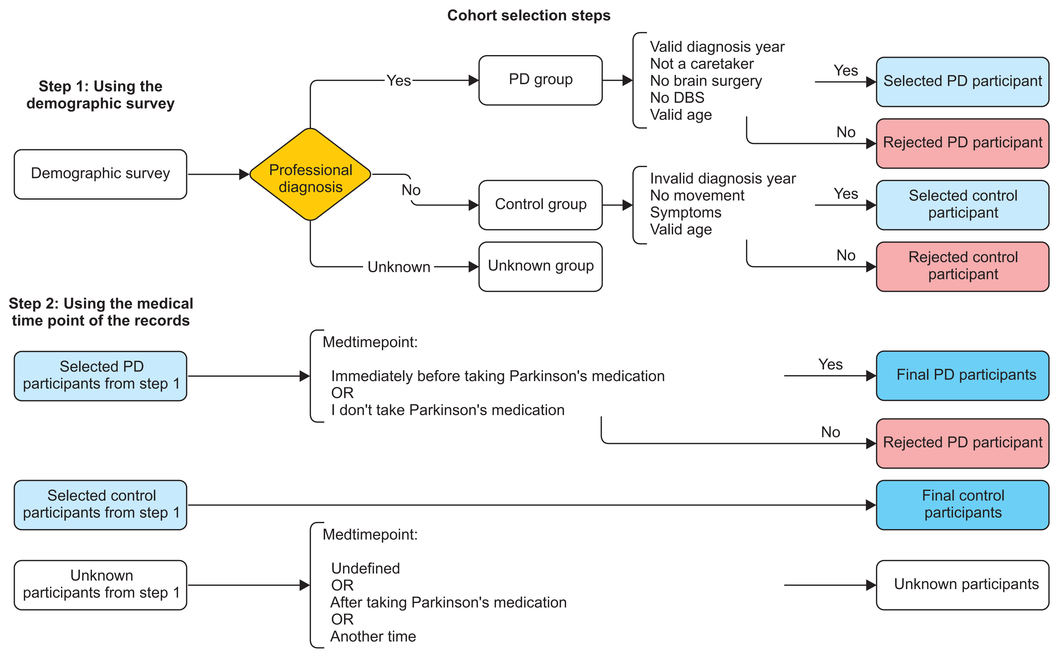
To avoid optimism in predicting PD, we conducted a serious cohort filtering process, which is illustrated in Figure 1 (steps 1 and 2).
Step 1: Using the demographic survey
  • - PD group selection: If the participant is professionally diagnosed by a doctor AND he or she has a valid date of diagnosis, AND is actually a Parkinsonian, not a caretaker, AND has never had surgery to treat PD nor deep brain stimulation, AND his or her age is valid.

  • - HC group selection: If the participant is not professionally diagnosed by a doctor, AND he or she has no valid date of diagnosis, AND has no movement symptoms, AND his or her age is valid.

  • - Unknown group selection: A participant is said to be unknown if their professional diagnosis is unknown.

Step 2: Using the medical time point of the recordings
The recordings were downloaded from [13] using the synapse Python client and SQL query commands, with a size of 80 GB. In this step, two important variables were used to filter the participants (healthCode from step 1 and medtime-point from this step); see Table 1 for details.
  • - PD group selection: Selected PD participants from step 1 AND (recordings of participants immediately before taking PD medication OR recordings of participants who didn’t take PD medication).

  • - HC group selection: The same participants from step 2.

  • - Unknown group selection: Unknown group from step 1 OR (records with undefined medication time point OR recordings of participants after taking PD medication OR recordings of participants at another time of the day).

Note AND represents the logical conjunction, OR represents the logical disjunction.
The final cohort dataset statistics are shown in Table 2.

2. Audio Signal Feature Extraction

Feature extraction is a primary step in ML and pattern recognition systems, particularly at the audio analysis stage. Audio signals are constantly changing, i.e., non-stationary, which is why, in most applications, audio signals are divided into short-term frames [15], and the analysis is done on a frame basis. Using the pyAudioAnalysis [16] library, we extracted important audio features that represented the properties of the selected recordings using two common techniques: the short-term and mid-term processing techniques.
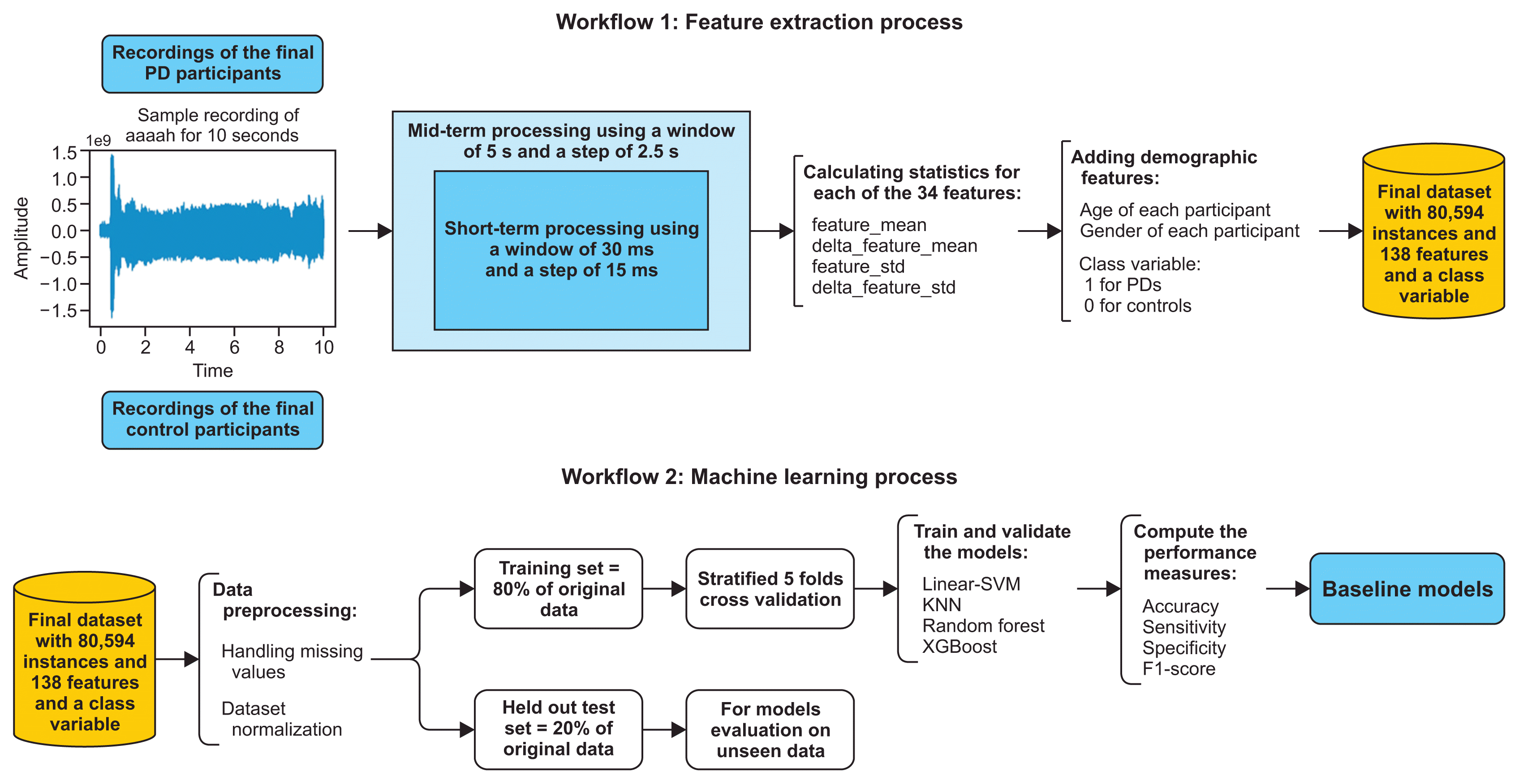
Short-term processing was done by following a windowing procedure. The window is generally between 20 ms and 40 ms [16]. Each recording was sampled at 44.1 kHz and divided into short windows of 30 ms with a step of 15 ms. The audio signal was multiplied with a shifted version of this window. This phase resulted in a sequence of feature vectors that led to 34 extracted features from the time, frequency, and cepstral domains [15,16] (Supplementary Table S1). The cepstral domain or the cepstrum is defined as the inverse discreet Fourier transform (DFT) of the log magnitude of the DFT of a signal.
The mid-term processing was done by dividing each recording into mid-term windows of 5 seconds (generally between 1 and 10 seconds [16]), with a step of 2.5 seconds. Then for each window, short-term processing was applied to calculate the feature statistics (feature_mean, delta_feature_mean, feature_std, delta_feature_std) for each of the 34 features. This resulted in 136 extracted audio features, plus the age and gender of each participant as well as the class variable (1 for PD participants, 0 for HC participants) (see workflow 1 in Figure 2). The final dataset had 80,594 instances, 138 features, and a class variable in total (Supplementary Table S2).

3. Baseline Models

Different techniques are better suited for different problems, and for different types of data (in our case predicting a category, with labeled data, under 100k samples). For this, we used the scikit-learn algorithm cheat-sheet [17] to select multiple classifiers that suited our problem, namely, linear-SVM, KNN, RF, and XGBoost.
The first step was to create a baseline ML model for each technique, using the default hyperparameters, and to compare their performance. To avoid overfitting, we used stratified 5-fold cross-validation because of our large dataset (+80k samples) although it was computationally intensive. Four measures were used to assess the performance of the classifiers, namely, accuracy, sensitivity, specificity, and the F1-score.
Before training our classifiers, we applied and compared various data preprocessing techniques. Data preprocessing is an important step in every ML process, including cleaning and standardization.

1) Dataset cleaning: handling missing values

It is quite common to have missing values in a dataset (NaNs). This was true in our case which resulted from the audio analysis feature extraction phase of some recordings. Handling missing values can improve an ML model’s accuracy. For this, we tested the following methods:
  • - Removing instances with missing values;

  • - Replacing missing values with zero;

  • - Imputing missing values with the mean, median, and most frequent value in each column.

2) Dataset normalization

Our dataset included features with different ranges, for example age between 18 and 85, gender either 0 or 1, zero crossing rate feature (zcr_mean) between 0 and 0.7, energy feature (energy_mean) between 6.205814e-09 and 5.019101e-01, and so on (Supplementary Table S1) for features description.
For this, dataset normalization was required to change the column values into a common range; hence, we implemented the following techniques:
  • - Dataset rescaling between 0 and 1 and between −1 and 1;

  • - Dataset normalization;

  • - Dataset standardization.

Then we compared the performance of those data processing techniques to choose the best combination to finally create the baseline models. We divided our dataset into a training set (80%) and held-out test set (20%). The test set was used to assess the performance of the final models on unseen data as seen in Figure 2 (workflow 2).

4. Feature Selection

Feature selection is one of the main concepts in ML. Having a large dataset increases the complexity of the models and may decrease their performance because it is computationally intensive. Various feature selection methods are widely used in the literature [18]. In this work, we adopted a filter method, and an embedded method. Wrapper methods were excluded due to their exhaustive search to find the optimal set of features that is computationally intensive, while using large datasets.

1) Filter method: ANOVA

ANOVA provides a statistical test to determine whether the means of several groups are equal. It computes the ANOVA F-value between each feature and the class variable. This F-value is used to select the subset of K features that have the strongest relationship with the class.

2) Embedded method: LASSO

LASSO is a regression analysis that performs L1 regularization which also performs an indirect feature selection. It has a parameter C that controls the sparsity; the smaller C, the fewer features are selected.
We decided to choose the maximum number of features in the 30th range to reduce the complexity of our models. In our case, adding less-important features (more than 30) made the classifiers more complex and did not add any significant or noticeable improvement in terms of performance. Thus, we tested various values of K(10, 20, 30) and C(0.01, 0.02, 0.03) to assess the performance of our classifiers, and decided on the best one (Table 3, Supplementary Table S3).

III. Results

1. Baseline Models Results

After preprocessing our dataset, using a combination of techniques that handle missing values and normalize the columns into a common range, deleting rows with missing values and rescaling the dataset between 0 and 1 gave the best performing baseline results. Table 4 presents the classification results obtained using all of the features. XGBoost was the most accurate, sensitive, and specific technique with 90.97%, 90.80%, and 91.14%, respectively, with an F1-score of 90.92%. Linear SVM was the least accurate, sensitive, and specific technique with 76.47%, 78.60%, and 74.36%, respectively, with an F1-score of 76.88%.

2. Feature Selection Results

Table 3 presents the classification results obtained after feature selection. We selected various subsets of ranked features using ANOVA’s K best parameter (K = 10, 20, and 30) and LASSO’s C parameter (C = 0.01, 0.02, and 0.03) and tested their performance for each ML technique.
RF was the most accurate, sensitive, and specific technique using ANOVA’s best 10, 20, and 30 features and using LASSO’s C = 0.01 and C = 0.02. KNN was the most accurate, sensitive, and specific technique using Lasso’s C = 0.03. Linear SVM was the least accurate, sensitive, and specific technique in all cases. Supplementary Table S3 presents the subset of features for each feature selection method using the various parameters K and C.

3. Hyperparameter Tuning Results

From Table 3, we concluded that the combination of features using LASSO outperformed ANOVA with almost the same number of features (K = 10 vs. C = 0.01, K = 20 vs. C = 0.02, K = 30 vs. C = 0.03). Thus, to perform hyperparameter tuning, we used the best subset of features that maximized the performance of each ML technique, knowing that the results shown in Table 4 were measured using the default hyperparameters with 138 features.
Linear SVM, KNN, and XGBoost were mostly accurate using LASSO and C = 0.03 with 76.02%, 92.69%, and 90.83%, respectively, using only 33 features. However, RF was mostly accurate using LASSO and C = 0.01 with 92.30% using only 11 features.
Table 5 presents the hyperparameter tuning results obtained using random search. XGBoost was the most accurate, sensitive, and specific technique with 95.31%, 95.19%, and 95.43%, respectively, with an F1-score of 95.28%, while predicting new cases on unseen data with an accuracy, sensitivity, and specificity of 95.78%, 95.32%, and 96.23%, respectively (Table 6) and with an F1-score of 95.74%. KNN, RF, and linear SVM were the least accurate, sensitive, and specific techniques.

IV. Discussion

This paper presented our method which we used to classify PD patients and distinguish them from HCs using 18,210 smartphone recordings by creating a dataset of 80,594 samples with 138 features and a class variable. The LASSO feature selection method outperformed ANOVA with almost the same number of features. From Supplementary Table S3, we conclude that age and gender features are highly ranked using both methods; it is known that PD is seen in people aged over 50, and it affects males more than females. Furthermore, energy entropy, spectral spread, and MFCC coefficients are highly ranked using both methods, which indicates the importance of extracting time, frequency, and cepstral domain features, in addition to the age and the gender of participants in classifying this disease.
From the same table, we can notice that there is a difference in the ranking of features between ANOVA and LASSO because each technique implements a different approach. ANOVA analyses the relationship between each feature and the class variable separately and assigns a test score to each feature. Then all the test scores are compared, and the features with top scores are selected (K = 10, 20, 30). On the other hand, LASSO regularization adds a penalty to the different parameters of the model to avoid overfitting. This penalty is applied over the coefficients that multiply each of the features. Thus, the L1 technique analyses all the features at once. In addition, LASSO has an important property of shrinking down to zero unimportant features, which depends on the chosen C parameter. For this reason, in Supplementary Table S3, there are different features for each C value in LASSO and the same ranked features using ANOVA with regards to the chosen K value. With this combination of features, XGBoost outperformed the remaining classifiers with an accuracy of 95.31% using 80% of the data (Table 5) while predicting new cases on unseen data with an accuracy of 95.78% (Table 6).
Several studies [1012] have reported high classification accuracy using SVM in the range of 91% to 93%, as seen in Table 7. However, in Tables 36, we note that SVM was the least accurate, with a maximum accuracy of 76.47% using 138 features. This is attributed to the fact that these studies used a small number of recordings, and small datasets. Furthermore, we found that a regular SVM takes time to fit the data (approximately 40 minutes). For this reason, we used linear SVM, which is optimized for large datasets, which limited our chances to test various other kernels (RBF, poly, and sigmoid).
Singh and Xu [19] used the same dataset that we used and achieved an accuracy of 99% using MFCC coefficients, L1-based feature selection, and an SVM classifier with an RBF kernel using 1,000 samples. The problem is that those 1,000 recordings were chosen randomly from an unbalanced database of 65,022 recordings, where 14% of participants were diagnosed with PD and 86% were healthy controls (claimed in their paper). Randomly choosing 1,000 recordings from an unbalanced set of recordings may have introduced an unbalanced set of 1,000 recordings. Moreover, those recordings were chosen without taking into account the medication time point; therefore, their dataset may have included some recordings of patients after they had taken PD medication. We avoided this in our cohort selection phase, as seen Figure 1, compared to our dataset where we made a 50/50% split of the recordings, where 9,105 were obtained from PD patients, and 9,105 were obtained from HCs. Furthermore, relying only on accuracy as a metric to assess the performance of the classifiers is not sufficient in medical diagnostic. Adding other metrics, such as sensitivity (which measures the proportion of PD patients that were correctly classified as having PD), and specificity (which measures the proportion of HCs that were correctly classified as not having PD) will give a better estimate of the performance of the classifiers. In our case, our highest classifier achieved an accuracy of 95.78%, a sensitivity of 95.32%, and a specificity of 96.23% with an F1-score of 95.74%. In the case of an unbalanced dataset (which is not clear in their case), relying only on accuracy may results in a high accuracy if one class is outnumbered; thus, introducing other metrics is important. Hence, we believe that our approach is more accurate and precise for classifying PD even if Singh et al. [19] achieved a higher accuracy which could be affected by their methodology choices.
In conclusion, we proposed a method to classify PD using a large sample of smartphone recordings as a sustained phonation of /a/ for 10 seconds. These recordings were then processed to extract multiple domain features in addition to demographic parameters to create an original dataset that was subjected to various ML techniques after data cleaning, normalization, and feature selection. We have demonstrated the importance of using these features to precisely classify PD with an accuracy of 95.78% using XGBoost. The main objective of this work was to build a smart framework based on ML techniques capable of distinguishing between PD patients and HCs using voice as a disease biomarker. As a future work, we aim to develop an mHealth system capable of implementing these ML techniques to speed up diagnosis time and to integrate it with conventional clinical methods.

Acknowledgments

The authors would like to thank every participant who contributed as a user of the Parkinson mPower mobile application and as part of the mPower study [13,14] developed by Sage Bionetworks and described in Synapse (https://doi.org/10.7303/syn4993293).

Notes

Conflict of Interest

No potential conflict of interest relevant to this article was reported.

Supplementary Materials

Supplementary materials can be found via https://doi.org/10.4258/hir.2020.26.4.274.

References

1. Parkinson J. An essay on the shaking palsy. London, UK: Sherwood, Neely and Jones;1817.
2. Parkinson J. An essay on the shaking palsy 1817. J Neuropsychiatry Clin Neurosci. 2002; 14(2):223–36.
3. Charcot JM. Lecon sur les maladies du systeme nerveux faites. Lesson on disease of the nervous system. Paris, France: Aux bureaux du Progres Medical;1872.
4. Charcot JM. Lectures on the diseases of the nervous system: delivered at La Salpetriere. London, UK: The New Sydenham Society;1877.
5. Brissaud E, Meige H. Lecons sur les maladies nerveuses (Salpetriere, 1893–1894). Paris, France: G. Masson;1895.
6. Heisters D. Parkinson’s: symptoms, treatments and research. Br J Nurs. 2011; 20(9):548–54.
crossref
7. Miller N, Allcock L, Jones D, Noble E, Hildreth AJ, Burn DJ. Prevalence and pattern of perceived intelligibility changes in Parkinson’s disease. J Neurol Neurosurg Psychiatry. 2007; 78(11):1188–90.
crossref
8. Ho AK, Iansek R, Marigliani C, Bradshaw JL, Gates S. Speech impairment in a large sample of patients with Parkinson’s disease. Behav Neurol. 1998; 11(3):131–7.
crossref
9. Tsanas A, Little MA, McSharry PE, Ramig LO. Accurate telemonitoring of Parkinson’s disease progression by noninvasive speech tests. IEEE Trans Biomed Eng. 2010; 57(4):884–93.
crossref
10. Little MA, McSharry PE, Hunter EJ, Spielman J, Ramig LO. Suitability of dysphonia measurements for telemonitoring of Parkinson’s disease. IEEE Trans Biomed Eng. 2009; 56(4):1015.
crossref
11. Benba A, Jilbab A, Hammouch A, Sandabad S. Voice-prints analysis using MFCC and SVM for detecting patients with Parkinson’s disease. In : Proceedings of 2015 International conference on electrical and information technologies (ICEIT); 2015 Mar 25–27; Marrakech, Morocco. p. 300–4.
crossref
12. Hemmerling D, Sztaho D. Parkinson’s disease classification based on vowel sound. In : Proceedings of the 11th International Workshop on Models and Analysis of Vocal Emissions for Biomedical Applications; 2019 Dec 17–19; Firenze, Italy.
13. Sage Bionetworks. mPower: mobile Parkinson disease study [Internet]. Seattle (WA): Sage Bionetworks;2019. [cited at 2020 Oct 29]. Available from: https://www.synapse.org/#!Synapse:syn4993293/wiki/247859 .
14. Bot BM, Suver C, Neto EC, Kellen M, Klein A, Bare C, et al. The mPower study, Parkinson disease mobile data collected using ResearchKit. Sci Data. 2016; 3:160011.
crossref
15. Giannakopoulos T, Pikrakis A. Introduction to audio analysis: a MATLAB approach. San Diego (CA): Academic Press;2014.
16. Giannakopoulos T. pyAudioAnalysis: an open-source python library for audio signal analysis. PLoS One. 2015; 10(12):e0144610.
crossref
17. Pedregosa F, Varoquaux G, Gramfort A, Michel V, Thirion B, Grisel O, et al. Scikit-learn: machine learning in Python. J Mach Learn Res. 2011; 12:2825–30.
18. Chandrashekar G, Sahin F. A survey on feature selection methods. Comput Electr Eng. 2014; 40(1):16–28.
crossref
19. Singh S, Xu W. Robust detection of Parkinson’s disease using harvested smartphone voice data: a telemedicine approach. Telemed J E Health. 2020; 26(3):327–34.
crossref

Figure 1
Cohort selection steps using the demographic survey and the medical timepoint of the records.
hir-26-4-274f1.gif
Figure 2
Feature extraction process and the machine-learning process. PD: Parkinson’s disease, SVM: support vector machine, KNN: k-nearest neighbor, XGBoost: extreme gradient boosting.
hir-26-4-274f2.gif
Table 1
Voice record variables
Variable Description
recordid This is a unique id for each record.
healthCode This is a unique id for each participant.
audio_countdown.m4a Recording of the environment for 5 seconds to verify that the microphone works.
audio_audio.m4a Voice recording of “aaaah” by the participant for 10 seconds.
medtimepoint This is a very important variable, which indicates when a participant records his voice:
Immediately before Parkinson medication OR
Just after Parkinson medication (at your best) OR
I don’t take Parkinson medications OR
AnotherTime
Table 2
Final cohort dataset statistics
PD group Control group
Number of selected recordings 9,105 9,105

Number of participants 453 1,037

Sex
 Male 280 836
 Female 173 201

Age (yr) 64.50 ± 8.16 (18–85) 53.62 ± 10.99 (18–85)

Values are presented number or mean±standard deviation (min–max).

Table 3
Performance of the four techniques using ANOVA and LASSO with various subsets of features
Method Parameter value Number of features Model Accuracy (%) Sensitivity (%) Specificity (%) F1-score (%)
ANOVA K = 10 10 Linear SVM 74.79 77.78 71.83 75.43
KNN 88.67 88.63 88.71 88.62
RF 92.09 91.77 92.42 92.03
XGBoost 89.33 88.94 89.72 89.24

K = 20 20 Linear SVM 74.53 77.72 71.37 75.23
KNN 89.49 89.16 89.82 89.41
RF 91.13 90.83 91.43 91.07
XGBoost 89.94 89.59 90.29 89.86

K = 30 30 Linear SVM 74.55 77.53 71.59 75.20
KNN 90.95 90.61 91.28 90.88
RF 91.42 91.07 91.77 91.35
XGBoost 90.59 90.49 90.92 90.54

LASSO C = 0.01 11 Linear SVM 74.38 77.29 71.50 75.02
KNN 89.54 89.54 89.55 89.50
RF 92.30 92.20 92.40 92.26
XGBoost 89.45 89.37 89.53 89.40

C = 0.02 21 Linear SVM 75.60 78.71 72.53 76.25
KNN 91.23 91.16 91.29 91.19
RF 92.29 92.15 92.43 92.25
XGBoost 90.38 90.13 90.64 90.38

C = 0.03 33 Linear SVM 76.02 78.80 73.26 76.58
KNN 92.69 92.38 92.99 91.59
RF 92.09 91.83 92.35 92.04
XGBoost 90.83 90.69 90.96 90.77

ANOVA: analysis of variance, LASSO: least absolute shrinkage and selection operator, SVM: support vector machine, KNN: knearest neighbor, RF: random forest, XGBoost: extreme gradient boosting.

Table 4
Performance of baseline models
Model Accuracy (%) Sensitivity (%) Specificity (%) F1-score (%)
Linear SVM 76.47 78.60 74.36 76.88
KNN 90.22 89.74 90.70 90.13
RF 89.88 88.77 90.98 89.72
XGBoost 90.97 90.80 91.14 90.92

SVM: support vector machine, KNN: k-nearest neighbor, RF: random forest, XGBoost: extreme gradient boosting.

Table 5
Optimal hyperparameters of models using random search
Machine learning technique Best feature selection method Optimal hyperparameters values Accuracy (%) Sensitivity (%) Specificity (%) F1-score (%)
Linear SVM Feature selection using LASSO with C = 0.03 penalty = l2
c = 92.82
verbose = false
dual = false
76.03 78.81 73.27 76.59
KNN Feature selection using LASSO with C = 0.03 n_neighbors = 1
weights = uniform
algorithm = kd_tree
leaf_size = 180
94.88 95.08 94.68 94.87
RF Feature selection using LASSO with C = 0.01 n_estimators = 1000
bootstrap = true
criterion = entropy
max_features = none
verbose = false
93.92 93.80 94.03 93.88
XGBoost Feature selection using LASSO with C = 0.03 n_estimators = 1000
max_depth = 15
learning_rate = 0.2
objective = binary:logistic
booster = gbtree
gamma = 0.5
min_child_weight = 3.0
subsample = 0.8
colsample_bytree = 0.9
colsample_bylevel = 0.9
reg_alpha = 0.1
silent = false
95.31 95.19 95.43 95.28

SVM: support vector machine, KNN: k-nearest neighbor, RF: random forest, XGBoost: extreme gradient boosting, LASSO: least absolute shrinkage and selection operator.

Table 6
Performance of the models on unseen data
Rank Model Accuracy (%) Sensitivity (%) Specificity (%) F1-score (%)
1 XGBoost 95.78 95.32 96.23 95.74
2 KNN 95.62 95.57 95.67 95.60
3 RF 94.52 94.19 94.84 94.47
4 Linear SVM 75.47 77.75 73.21 75.93

SVM: support vector machine, KNN: k-nearest neighbor, RF: random forest, XGBoost: extreme gradient boosting.

Table 7
Comparison of our methodology with other studies
Study Dataset Methodology Results
Little et al. [10] They used an original dataset consisting of 195 recordings collected from 31 patients where 23 were diagnosed with PD They detected dysphonia by discriminating HCs from PD participants, by extracting time domain and frequency domain features They achieved an accuracy of 91.4% using SVM classifier with 10 highly uncorrelated measures.
Benba et al. [11] They used a dataset consisting of 17 PD patients and 17 HCs They classified PD participants from HCs using a set of recordings recorded using a computer’s microphone, and by extracting 20 MFCC coefficients They achieved an accuracy of 91.17% using linear SVM with 12 MFCC coefficients.
Hemmerling et al. [12] They used an original dataset consisting of 198 recordings collected from 66 patients where 33 were diagnosed with PD They extracted several acoustic features, and applied Principal Component Analysis (PCA) for feature selection They achieved and accuracy of 93.43% using linear SVM
Singh and Xu [19] They selected randomly 1,000 recordings from the mPower database They extracted MFCC coefficients using the python_speech_ features library and compared different feature selection techniques They achieved an accuracy of 99% using SVM with an RBF kernel and by selecting important features using L1 feature selection technique
This study We have used a set of 18,210 smartphone recordings from the mPower database where 9,105 recordings are of PD participants and 9,105 recordings are of healthy controls We have extracted several features, from time frequency and cepstral domains, we have applied different preprocessing techniques and used two feature selection methods ANOVA and LASSO to compare Four different classifiers using 5-fold cross-validation We have achieved on unseen data a high accuracy, sensitivity, and specificity of 95.78%, 95.32%, and 96.23% respectively, and an F1-score of 95.74% using XGBoost with 33 features out of 138 that were chosen using LASSO with C = 0.03

HC: health control group, PD: Parkinson’s disease, SVM: support vector machine, MFCC: mel-frequency cepstral coefficients, RBF: radial basis function, LASSO: least absolute shrinkage and selection operator.

TOOLS
Similar articles