

 PDF
PDF Citation
 Print
Print


INTRODUCTION
PARAMETRIC MAPPING
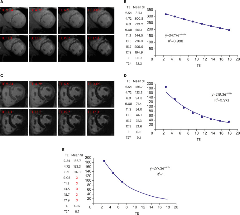 | Figure 1T2* imaging to assess myocardial iron overload. (A) T2* scan of a normal heart showing slow signal loss with increasing TE. (B) Decay curve for normal heart (T2*=33.3 ms). (C) Heavily iron overloaded heart. Note there is substantial signal loss at TE = 9.09. (D) Decay curve for heavily iron overloaded heart showing rapid signal loss with increasing TE. The curve plateaus as myocardial signal intensity falls below background noise. (E) Values for higher TEs are removed (truncation method) resulting in a better curve fit and a lower T2* value. As originally published by BioMed Central in Schulz-Menger et al. Journal of Cardiovascular Magnetic Resonance 2013;15:35.3)TE = echo time.
|
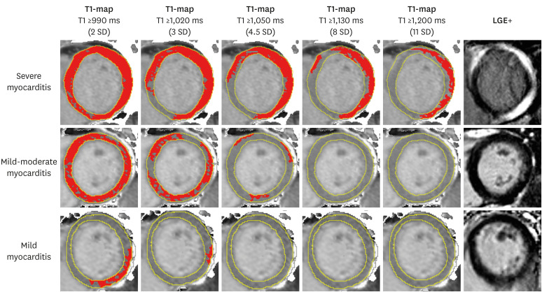 | Figure 2T1-maps using incremental thresholds demonstrate the predominantly non-ischemic pattern of injury across a spectrum of acute myocarditis. Red indicates areas of myocardium with a T1 value above the stated threshold of at least 40 mm2 in contiguous area. T1 threshold of 990 ms was previously validated for the detection of acute myocardial edema; other thresholds were selected for illustrative purposes. As originally published by Biomed Central in Ferreira et al. Journal of Cardiovascular Magnetic Resonance 2014;16:36.4)LGE = late gadolinium enhancement; SD = standard deviation.
|
T1-MAPPING
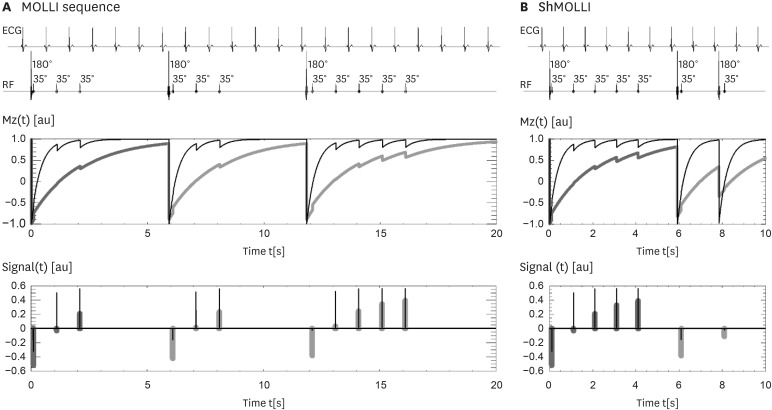 | Figure 3ECG-gated pulse sequence schemes for simulation of (A) MOLLI and (B) ShMOLLI at a heart rate of 60 bpm. SSFP readouts are simplified to a single 35° pulse each, presented at a constant delay time TD from each preceding R wave. The 180° inversion pulses are shifted depending on the IR number to achieve the desired first TI of 100, 180 and 260 ms in the consecutive IR experiments. The plots below represent the evolution of longitudinal Mz for short T1 (400 ms, thin lines) and long T1 (2,000 ms, thick lines). Note that long epochs free of signal acquisitions minimise the impact of incomplete Mz recoveries in MOLLI so that all acquired samples can be pooled together for T1 reconstruction. In ShMOLLI the validity of additional signal samples from the 2nd and 3rd IR epochs is determined by progressive nonlinear estimation. As originally published by BioMed Central in Piechnik S et al. Journal of Cardiovascular Magnetic Resonance 2010;12:69.10)IR = inversion recovery; MOLLI = modified Look-Locker inversion recovery; Mz = longitudinal magnetization; ShMOLLI = shortened modified Look-Locker inversion recovery; SSFP = steady-state free precession; TD = trigger delay.
|
Native T1-mapping
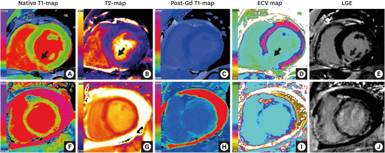 | Figure 4CMR mapping and LGE imaging in acute myocardial pathologies. (Top row) CMR (3 Tesla) images of a patient with an acute myocardial infarction in the inferior septum. (A) Native T1-map (ShMOLLI) showing significantly increased T1 values in the inferior septum (1,407 ms vs. 1,159 ms in remote myocardium in the anterior wall; normal ShMOLLI T1 at 3T = 1,166±60 ms). (B) T2-map showing increased T2 values in the inferior septum (arrow, 55 ms vs. 39 ms in remote myocardium in the anterior wall). (C) Post-gadolinium contrast T1-map. (D) ECV map showing significantly increased ECV in the inferior septum (59% vs. 30% in remote myocardium in the anterior wall). (E) LGE imaging showing transmural enhancement with a core area of microvascular obstruction in the inferior septum (arrow). (Bottom row) CMR (1.5 Tesla) images of a patient with acute myocarditis. (F) Native T1-mapping using the ShMOLLI method showed significantly increased global myocardial T1 values (1,060 ms; normal ShMOLLI T1 at 1.5T = 962±25 ms). (G) T2-map showed increased global myocardial T2 values (59 ms), consistent with edema. (H) Post-gadolinium contrast T1-map. (I) ECV mapping showed increased global ECV of 36% (normal 27±3%). (J) LGE imaging showed small areas of patchy enhancement in a non-coronary distribution.CMR = cardiovascular magnetic resonance; ECV = extracellular volume; LGE = late gadolinium enhancement; ShMOLLI = shortened modified Look-Locker inversion recovery.
|
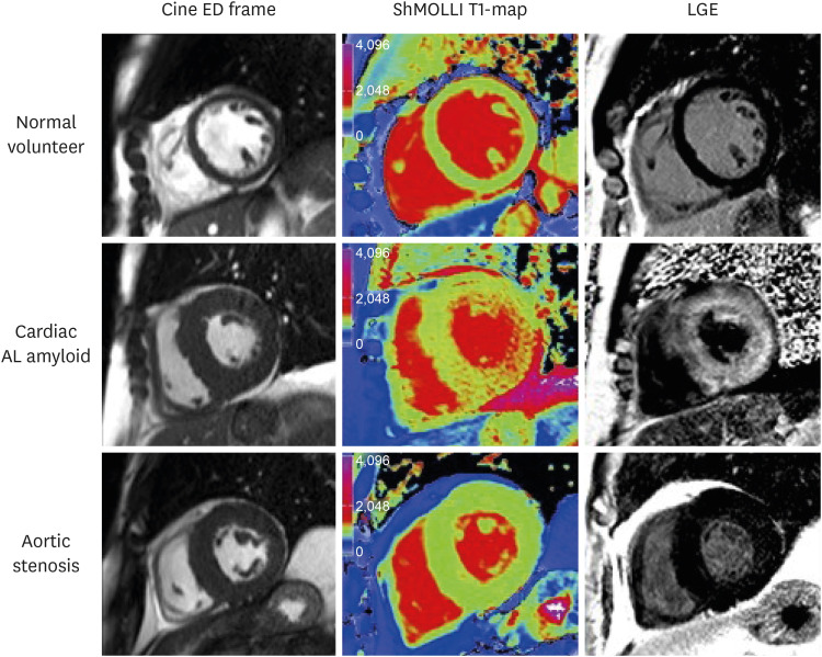 | Figure 5Characteristic examples from CMR scans. CMR end-diastolic frame from cine (left panel), ShMOLLI non-contrast T1 map (middle panel), and LGE images (right panel) in normal volunteer, aortic stenosis patient, and cardiac amyloid patient. Note the markedly elevated myocardial T1 time in the cardiac amyloid patient (1,170 ms, into the red range of the color scale) compared to the normal control (955 ms) and the patient with aortic stenosis and left ventricular hypertrophy (998 ms). As originally published in Karamitsos et al. JACC: Cardiovasc Imaging 2013;6:488-97.17)AL = amyloid light chain; CMR = cardiovascular magnetic resonance; ED = end diastolic; LGE = late gadolinium enhancement; ShMOLLI = shortened modified Look-Locker inversion recovery.
|
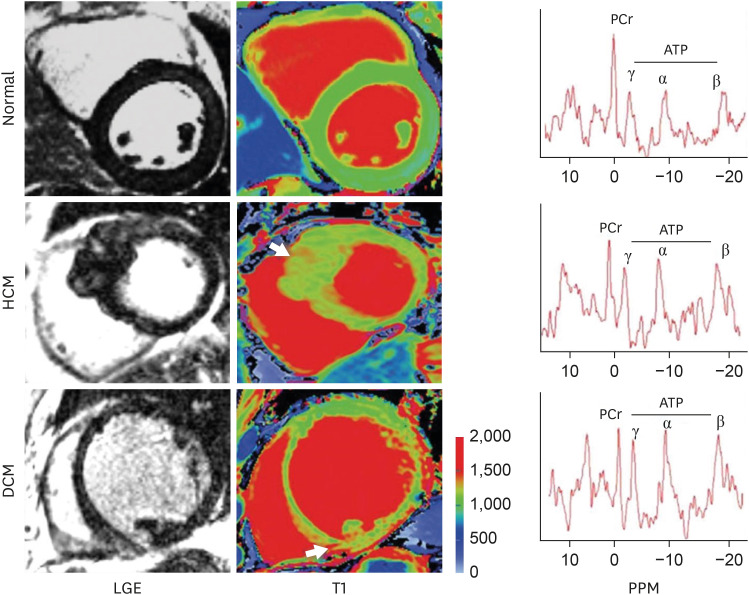 | Figure 6LGE and T1 images in normal, HCM, and DCM. Arrows point to focal areas of LGE and high T1. Note: There is diffusely high T1 in the septum of HCM and inferior septum/inferior in the DCM. Representative spectra for each condition are shown; PCr indicates phosphocreatine; and ATP adenosine triphosphate. As originally published in Dass S. et al. Circulation Cardiovascular Imaging 2012;5:726-33.30)ATP = adenosine triphosphate; DCM = dilated cardiomyopathy; HCM = hypertrophic cardiomyopathy; LGE = late gadolinium enhancement; PCr = creatine phosphate.
|
Post-contrast T1-mapping and ECV
Stress T1-mapping
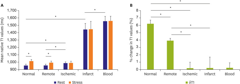 | Figure 7Myocardial T1 at rest and during adenosine stress at 1.5-T. (A) T1 values at rest in normal and remote tissue were similar and significantly lower than in ischemic regions. Infarct T1 was the highest of all myocardial tissue, but lower than the reference left ventricular blood pool of patients. During adenosine stress, normal and remote myocardial T1 increased significantly from baseline, while T1 in ischemic and infarcted regions remained relatively unchanged. (B) Relative T1 reactivity (δT1) in the patient's remote myocardium was significantly blunted compared to normal, and completely abolished in ischemic and infarcted regions. All data indicate mean ±1 SD. Adapted from Liu et al. JACC: Cardiovascular Imaging 2016;9:27-36 originally published by Elsevier.35)SD = standard deviation.
*p<0.05.
|
T2-MAPPING
IMAGING PROTOCOL
T1-mapping
1) Native T1 mapping is performed in the absence of contrast or stress agents, at rest.
2) Look Locker imaging (MOLLI or ShMOLLI10) or equivalent) should be used.
3) Diastolic acquisition is best with the exception of atrial fibrillation in which systolic acquisition may be preferred. In patients with higher heart rates, specific sequences designed for these heart rates should be used.
4) Source images should be checked for motion/artefact and imaging repeated if this occurs. If motion correction is used, this needs to be carefully checked for introduction of any new artefacts.46)
5) Slice thickness: 6–8 mm, in-plane resolution ~1.6–2.0 mm
6) The number and orientation of slices obtained will depend upon the indication. At least one short-axis (SA) map should always be obtained.
7) For extracellular volume measurements, T1 mapping should be performed prior to contrast and at least 1 time point between 10 and 30 minutes post contrast bolus. Post-contrast T1-maps should match native T1-maps in slice position and other prescribed imaging parameters (such as field of view and cardiac phase).
8) The hematocrit should be measured just before the scan and, ideally within 24 h of imaging, for the accurate ECV fraction measurement.
T2-mapping
1) Multiple alternatives exist, such as T2-prepared single-shot bSSFP sequence acquired with different T2 prep time, GraSE or FSE-based pulse sequences.
2) Slice thickness: 6–8 mm, in plane-resolution ~ 1.6–2.0 mm
3) Diastolic acquisition is recommended.
4) The number and orientation of slices obtained will depend upon the indication. SA maps should always be obtained.
5) Source images should be checked for motion/artefact, including in motion-corrected images, and imaging repeated if this occurs.
Example CMR parametric mapping protocol
• Localizers
• Pilot scouts
• Cine imaging (horizontal long-axis [HLA], vertical long-axis [VLA], left ventricular outflow tract [LVOT])
• Native T1 mapping
• T2 mapping
• T2* imaging
• Injection of gadolinium-based contrast agents for LGE imaging
• Cine imaging (SA stack)
• LGE (HLA, VLA, LVOT, SA stack)
• Wait at least 10 minutes post-GBCA to acquire post-contrast T1-maps for ECV quantification
IMAGE POST-PROCESSING AND ANALYSIS
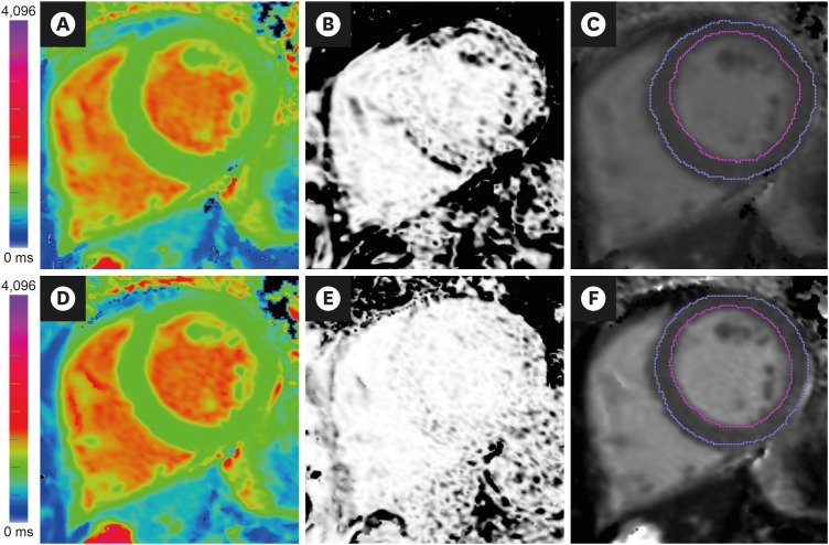 | Figure 8Image analysis of T1-maps. (A) Native T1-map (ShMOLLI at 1.5 Tesla). The acquisition of this T1-map suffered from breathing motion, resulting in (B) an R2 map that showed poor T1 fit (black pixels within the LV myocardium) and (C) underestimated average LV myocardial T1 values (T1=928 ms) after myocardial segmentation using epi- and endo-cardial contours (blue and magenta lines). Guided by the suboptimal R2 map, the operator repeated the acquisition with the patient performing a good breath-hold, which produced (D) A good quality native T1-map, as indicated by (E) an R2 map that showed good T1 fit (pixels within the LV myocardium are white), and (F) accurate average LV myocardial T1 values (T1=943 ms). Ensuring good data fit during image acquisition and analysis is paramount in the clinical application of mapping techniques.LV = left ventricular; ShMOLLI = shortened modified Look-Locker inversion recovery.
|
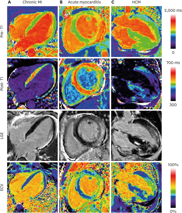 | Figure 9Examples illustrating excellent agreement between LGE and ECV in cases of focal abnormalities in myocardial ECV. Pre-contrast T1-maps (top row), post-contrast T1-maps (2nd row), late gadolinium enhancement (3rd row), and ECV maps (bottom row) for patients with: (A) chronic MI, (B) acute myocarditis, and (C) HCM. As originally published by BioMed Central in Kellman et al. Journal of Cardiovascular Magnetic Resonance 2012;14:64.51)ECV = extracellular volume; HCM = hypertrophic cardiomyopathy; LGE = late gadolinium enhancement; MI = myocardial infarction.
|
REPORTING
1) For clinical reports, the type of pulse sequence, reference range, and type/dose of gadolinium contrast agent (if applied) should be quoted.
2) Mapping results should include the numerical absolute value, the Z-score (number of standard deviations by which the result differs from the local normal mean; if available), and the normal range of the CMR system.
3) Local results should be benchmarked against published reported ranges, but a local reference range should be primarily used.
4) Reference ranges should be generated from data sets that were acquired, processed, and analyzed in the same way as the intended application, with the upper and lower range of normal defined by the mean ±2 SD of the normal data, respectively.
5) Parameter values should only be compared to other parameter values if they are obtained under similar conditions. In other words, the acquisition scheme, field strength, contrast agent and processing approach should be the same, and the results should be reported along with corresponding reference ranges for the given methodology.
In addition to the above, the authors also recommend including the following:
6) Recording the quality of T1/T2 maps before using for clinical diagnosis, via assessment of T1/T2 curve-fits and/or quality controls maps (such as R2 or residual maps)
7) Report the number of slices obtained and their imaging plane prescription (e.g. 3 SA slices covering the LV)
8) Consistent and standardized training of image analysis and post-processing of parametric maps48)
9) In additional to global T1/T2 values, the extent of any regional abnormalities based on segmental analysis, and the range of these values (e.g. “The basal-mid inferolateral segments have areas with significantly elevated T1 values, ranging from 1,000–1,050 ms”)
10) An interpretation or differential diagnosis of the imaging findings within the clinical context of the referral (e.g. “…which may be consistent with acute myocardial inflammation in these areas”)
 XML Download