Factors Associated with 5-Year Costs of Care among a Cohort of Alcohol Use Disorder Patients: A Bayesian Network Model

Elina Rautiainen; Olli-Pekka Ryynänen; Tiina Laatikainen; Pekka Kekolahti

doi:10.4258/hir.2020.26.2.129

Journal List > Healthc Inform Res > v.26(2) > 1144856

Go to TopGo to Top Go to BottomGo to Bottom

TOOLS

Rautiainen, Ryynänen, Laatikainen, and Kekolahti: Factors Associated with 5-Year Costs of Care among a Cohort of Alcohol Use Disorder Patients: A Bayesian Network Model

Original Article

Healthcare Informatics Research 2020; 26(2): 129-145.

Published online: 30 April 2020

DOI: https://doi.org/10.4258/hir.2020.26.2.129

Factors Associated with 5-Year Costs of Care among a Cohort of Alcohol Use Disorder Patients: A Bayesian Network Model

Elina Rautiainen^1,²

, Olli-Pekka Ryynänen^1,³

, Tiina Laatikainen^1,^2,⁴

, Pekka Kekolahti⁵

¹Department of Public Health and Clinical Nutrition, University of Eastern Finland, Kuopio, Finland

²Finnish Institute for Health and Welfare, Helsinki, Finland

³General Practice Unit, Kuopio University Hospital, Primary Health Care, Kuopio, Finland

⁴Joint Municipal Authority for North Karelia Social and Health Services (Siun sote), Joensuu, Finland

⁵Department of Communications and Networking, School of Electrical Engineering, Aalto University, Espoo, Finland

Corresponding Author: Elina Rautiainen, Department of Public Health and Clinical Nutrition, University of Eastern Finland, PO Box 1627, FI-70211 Kuopio, Finland. Tel: +358503103519, E-mail: elinara@uef.fi (https://orcid.org/0000-0001-6942-0845)

Received 29 January 2020 Revised 23 March 2020 Revised 14 April 2020 Accepted 16 April 2020

This is an Open Access article distributed under the terms of the Creative Commons Attribution Non-Commercial License (http://creativecommons.org/licenses/by-nc/4.0/) which permits unrestricted non-commercial use, distribution, and reproduction in any medium, provided the original work is properly cited.

Abstract

Objectives

To examine the direct effects of risk factors associated with the 5-year costs of care in persons with alcohol use disorder (AUD) and to examine whether remission decreases the costs of care.

Methods

Based on Electronic Health Record data collected in the North Karelia region in Finland from 2012 to 2016, we built a non-causal augmented naïve Bayesian (ANB) network model to examine the directional relationship between 16 risk factors and the costs of care for a random cohort of 363 AUD patients. Jouffe’s proprietary likelihood matching algorithm and van der Weele’s disjunctive confounder criteria (DCC) were used to calculate the direct effects of the variables, and sensitivity analysis with tornado diagrams and analysis maximizing/minimizing the total cost of care were conducted.

Results

The highest direct effect on the total cost of care was observed for a number of chronic conditions, indicating on average more than a €26,000 increase in the 5-year mean cost for individuals with multiple ICD-10 diagnoses compared to individuals with less than two chronic conditions. Remission had a decreasing effect on the total cost accumulation during the 5-year follow-up period; the percentage of the lowest cost quartile (42.9% vs. 23.9%) increased among remitters, and that of the highest cost quartile (10.71% vs. 26.27%) decreased compared with current drinkers.

Conclusions

The ANB model with application of DCC identified that remission has a favorable causal effect on the total cost accumulation. A high number of chronic conditions was the main contributor to excess cost of care, indicating that comorbidity is an essential mediator of cost accumulation in AUD patients.

Go to :

Keywords: Bayes Theorem, Causality, Alcohol-Related Disorders, Health Care Costs, Costs and Cost Analysis

I. Introduction

Alcohol use disorders (AUDs) are characterized as chronic and relapsing conditions associated with high cost of care [1–3]. The overall economic burden of AUDs is remarkable, varying between 40 and 58 billion euros (€) in Europe [4,5].

The clinical course and prognosis of AUD in treated samples are known to be affected by several factors, including severity of the AUD, demographic and socio-economic factors, and mental health comorbidity [6–9], and long-term abstinence rates in treated populations vary only around 5.8% [10,11]. However, long-term studies on predictors of the future cost accumulation across social and healthcare service systems among this patient group have found mixed results, especially regarding the role of achieving stable remission [12–14]. Age, gender, employment status, co-occurring mental health problems, and abstinence status have all been associated with healthcare cost accumulation among individuals with AUD [14,15].

Electronic Health Records (EHRs) provide extensive information on individual health, and the performance of the treatment system and machine learning techniques have proved to be useful in predictive modeling based on these data [16–20]. Research on predicting healthcare costs in high-need patients is also gaining interest [21]. However, there has still been very little research regarding the causal links and direct effects between various risk factors and treatment costs among high-need AUD patients.

In this study, we aimed to identify the causal associations of various socio-economic and health-related factors with the 5-year cost of care for a clinical cohort of AUD patients. The specific aim was to assess the causal effect of AUD remission on the cost of care. We hypothesized that remission has a cost decreasing effect. We further produced a profile of independent variables’ values maximizing and minimizing costs during 5 years of follow-up, based on sensitivity analysis (SA) among variables.

Go to :

II. Methods

1. Sample

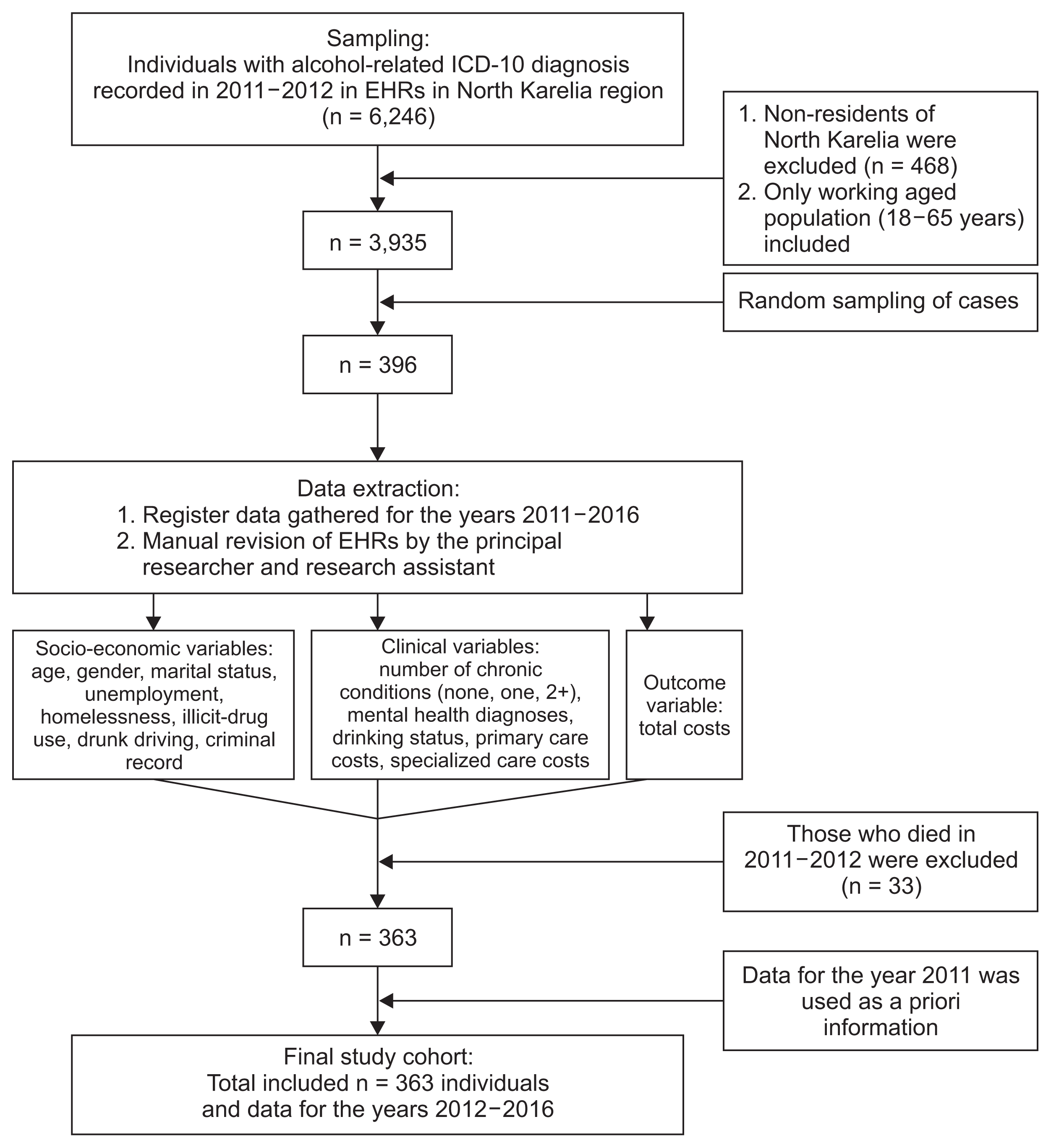
To examine the magnitude of 16 risk factors on cost accumulation, we used a random sample (n = 363) of AUD patients identified through EHRs based on alcohol-related ICD-10 (the International Statistical Classification of Diseases and Related Health Problems, 10th revision) codes. Figure 1 presents the research flow. The study cohort was randomly sampled from the regional EHR system in the North Karelia region in Finland based on the following alcohol-related ICD-10 diagnosis codes: G312, G405, G4050, G4051, G4052, G621, I426, K292, F100, F101, F102, F103, F104, F105, F106, F108, F109, K860, K700, K701, K702, K703, K704, K709, T510, T511, T512, T513, T518, T519, X45, and X69 (see Appendix 1 for more detailed information). Retrospective sampling included the years 2011 and 2012. Of the identified overall AUD population of (n = 6,246) individuals, we first formed a random cohort of 396 individuals by using Excel random sampling, and their health service use cost data were retrieved from the EHRs for the years from 2011 to 2016. We then excluded individuals who died or remitted in 2011 because we were not able to explicitly identify which costs in 2011 were caused before remission and which were caused after. Thus, the final study sample included 363 individuals. Based on the manual assessment of the EHR data conducted by two reviewers, the principal researcher and research assistant, we identified that the cohort represented individuals with a severe form of AUD. AUD was defined according to the Diagnostic and Statistical Manual of Mental Disorders (DSM-V) and ICD-10 to include both harmful use and alcohol dependence.

Figure 1

Diagram of sampling and data extraction process. ICD-10: the 10th revision of the International Statistical Classification of Diseases and Related Health Problems, EHR: Electronic Health Record.

2. Measurement

The examined outcome was the total cost of care. Data on the cost of care were used for the years from 2012 to 2016, and cost data from 2011 were used as a priori information. Specialized care costs were retrieved from the hospital EHR system, including all hospitalizations, outpatient visits and admissions, and their costs derived from the hospital’s cost accounting systems. Primary care costs were retrieved from the outpatient EHR system but were underestimates of the true costs, as the primary care database did not include e.g. private health service use costs (see Appendix 2 for more information). Total costs were discretized to quartiles. In the assessment of the causal effect of AUD remission on patients’ costs of care, those with continual AUD were used as a reference, and those who died before the year 2012 were excluded from analysis.

We identified 16 factors associated with AUD trajectories and their costs based on the literature [14,15,22], including socioeconomic variables encompassing age, gender, marital status, unemployment status, and social problems like homelessness, illicit drug use, criminal record, and drunk driving. Data on drinking status and socioeconomic variables were manually collected from EHRs and the municipal social services database mainly as dichotomous variables. In addition, clinical variables included the number of ICD-10 diagnoses of chronic conditions (i.e., permanent diagnoses). Diagnoses were classified into three groups, according to number: (1) none, (2) one, and (3) two or more. Mental health diagnoses included ICD-10 codes F00 to F99 (mental and behavioral disorders), excluding F10 codes. Drinking status was defined as continual AUD or stable AUD remission. Stable remission was defined as sustained abstinence or managed use that lasted until the end of the follow-up period, with a minimum duration of 6 months. Time estimate in AUD remission was based on health professionals’ objective notes and diagnosis information. Individuals with any shorter abstinence periods were included in the continual AUD group.

3. Ethical Considerations

The study was approved by the Research Ethics Committee of the Northern Savo Hospital District (No. IRB00006251). Consent was not obtained, as the study was based on registry information. Patients were not contacted.

4. Statistical Analysis

We performed the statistical analysis using the Bayesian network approach with the BayesiaLab 9.0 tool [23]. The visual form of a Bayesian network is a directed acyclic graph (DAG), from which direct and indirect effects, common causes, and effects can be discovered and mathematically expressed. A DAG consists of nodes presenting random variables X_i, and arcs or lines presenting associations between a pair of variables. A DAG defines a factorization of joint probability of a Bayesian network into a product of local probability distributions, one for each variable:

$P (X_{1}, \dots, X_{n}) = \prod_{i = 1}^{n} P (X_{i} | p a_{X i}),$

where pa_Xi are parents of a variable X_i. This type of representation enables both deductive and abductive inference from the model, allowing fixing of (controlling for) one or several variables’ probability distributions for inference of the direct or total effect of the variables of interest on the target variable.

Bayesian networks are used for both non-causal (predictive or explanatory) and causal modeling. In the non-causal model, the arc describes probabilistic relationships between the parent variable(s) and the child variable(s), whereas in the causal model it describes the existence of a direct causal dependence between two variables. A Bayesian network structure is constructed by using a bottom-up modeling approach (i.e., using structural and parameter learning from data), a top-down approach (i.e., manual construction based on existing expert knowledge), or a hybrid of the bottom-up and top-down methods. Multiple algorithms exist for structural learning. A supervised learning method with a minimum description length (MDL) score [24] uses a naive structure, such as augmented naive Bayesian (ANB) and tree augmented naive Bayesian (TAN), whereas an unsupervised learning method uses greedy search (e.g., maximum spanning tree, taboo, and hill climbing) with MDL scoring to construct a non-naive Bayesian network. Supervised learning is used mainly for predictive modeling, and unsupervised learning is adapted for clustering and for the construction of a causal Bayesian network. However, human intervention is required to verify the correctness of causal directions.

The MDL score optimizes the model complexity against the model fit to data and can be expressed at a high level as

$MDL (BN, Data) = DL (Data | BN) + SC * (DL (G) + DL (CPT | G)),$

where BN is a Bayesian network including parameters, DL is a description length in bits, G is the graph part of a BN, CPTs are conditional probability tables for each variable X_i in the model, and SC is the structural coefficient. With the SC, the effect of the complexity of the network to the score can be increased (SC < 1) or decreased (SC > 1). A more detailed level MDL equation is provided in Appendix 3.

A true causal network between the variables and the target variables is hard to estimate. Especially in settings with numerous variables, information of a complete causal structure is often unknown. Nevertheless, causality can be estimated by applying van der Weele and Shiptser’s modified disjunctive confounder criteria (DCC) for calculating the direct causal effect of a variable on the target variable from a non-causal Bayesian network [25,26]. According to the DCC, correctly selected confounders are the key for successful blocking of all backdoor and frontdoor paths between the treatment and the target variables in a Bayesian network. Van der Weele and Shiptser [25] defined the original DCC as “controlling for each variable that is a cause of the treatment, or of the target, or both”. Van der Weele [26] added two additional qualifications to the DCC for practical use for confounder controlling and re-named it the modified disjunctive confounding criterion, called in this article modified DCC. Additional definitions are (1) discarding any variable known to be an instrumental variable and (2) including variables that do not satisfy criteria but are good proxies for unmeasured common causes of treatment.

Continuous variables were discretized using a convenience distribution for the variable age with 10-year intervals. The variables implying costs were discretized to quarters having 25% of observations in each class. The outcome variable was cumulative healthcare costs (totalcost_2012–2016), which was discretized into equal quartiles, qualitatively described as “low cost” (≤€4,486.54), “medium cost” (€4,486.55–€15,746.10), “high cost” (€15,746.11–€46,864.36), and “very high cost” (€46,864.37–€1,180,863.75).

Supervised ANB learning was used in the study to construct a Bayesian network. To find the optimal complexity of the model in the ANB learning phase, an SC analysis was performed as part of MDL scoring, and the value SC = 0.6 was used in the analysis.

The result was a non-causal ANB network model with 16 independent variables. BayesiaLab allows every variable and their combinations to be fixed to certain values. For example, the variable “status2012” can be fixed to the value “remitted” = fixed to 100%. Then the model gives the values of the outcome in that hypothetical case that individuals had an AUD remission. We analyzed the probabilistic effect of independent variables by fixing each variable’s values separately to be 100%.

Following the modified DCC, we examined the effect of AUD remission in 2012 (continuous drinking vs. remission) by fixing marginal distributions of all other independent variables except drinking status (status2012). We analyzed the variables associated with the variable status2012 (continuous AUD/AUD remission) by a semi-structured search with status2012 as the target. The following variables were associated with status2012: drug use (strongest effect), homelessness, criminal background, gender, marital status, and income support, fulfilling the criteria of the DCC. In a similar analysis, we found the following variables to be associated with the outcome totalcost_2012–2016: number of somatic diagnoses, age, income support, municipality, and specialized care costs 2011. The variable “income support” was the only variable associated with both the outcome and index variable status2012. We also used the variable “number of psychiatric diagnoses” in ANB modeling for a measurement of psychiatric background.

We used Jouffe’s proprietary likelihood matching (PLM) algorithm, which implements the modified DCC and allowed us to estimate the independent variables’ causal effect on the target while holding others constant [27].

An SA among variables allows the identification of combinations of variable values that have the maximum or minimum effect on the target variable. SA was performed twice using hard evidence, showing first the maximum and then the minimum effect on costs (target variable totalcost_2012–2016).

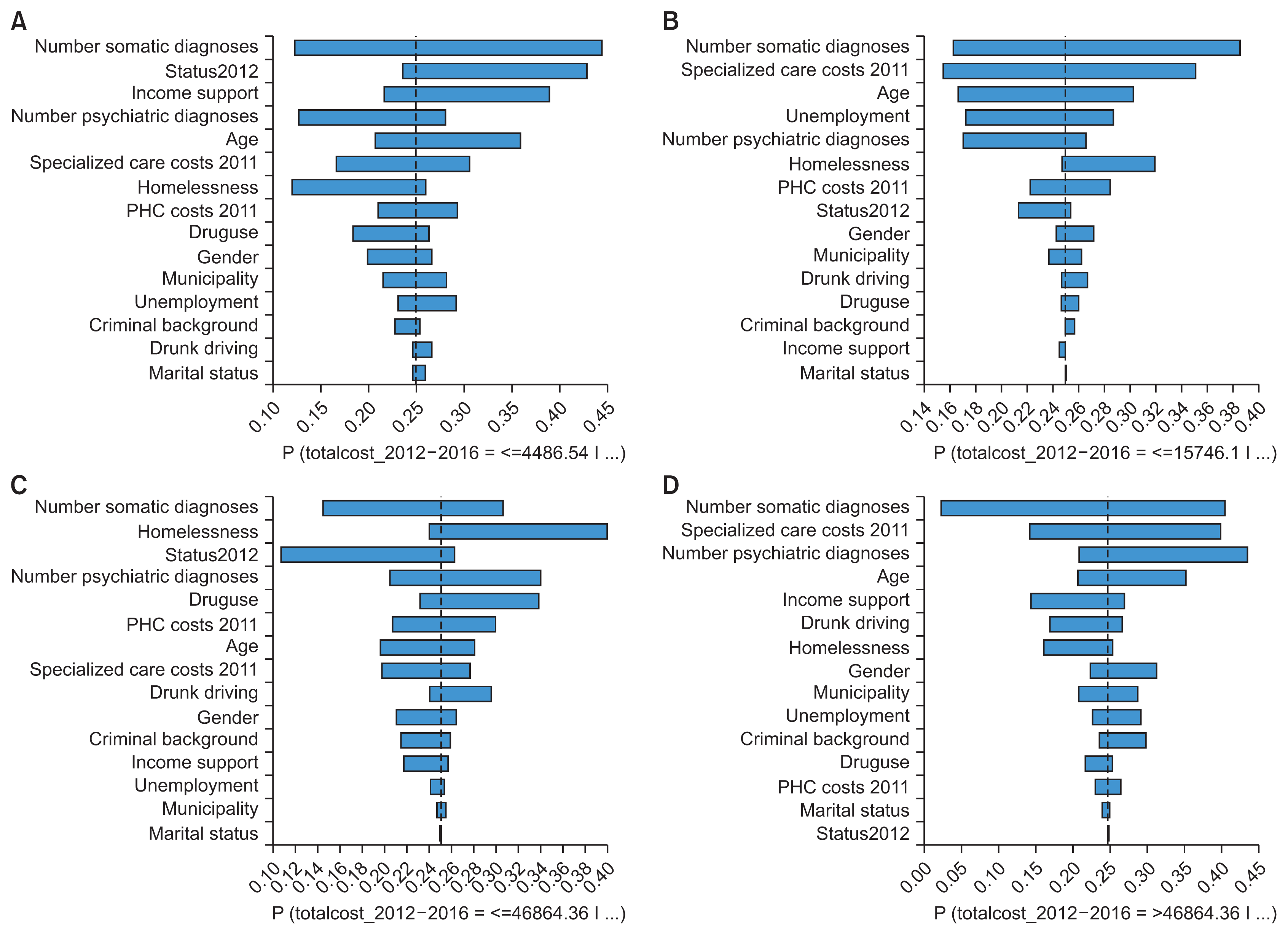
A tornado diagram is a design for SA. The diagram consists of two-sided horizontal bars to visualize the factors with the largest impact (positive or negative) on the outcome variable. The widest bar showing the largest impact is placed at the top. Bars to the right of the midline show the positive effect on the outcome variable, whereas bars to the left represent a negative effect. The diagram is presented separately for each value of the outcome variable.

Go to :

III. Results

The dataset with discretization of numerical variables is presented in Table 1. Until the end of 2016, 62.8% continued drinking, 16.5% died, and 20.7% remitted. The research data contained 335 missing values (4.2% of the dataset), whose type was missing at random. We input the missing values by using an expectation-maximization algorithm. The predictive performance of the model as an area under ROC curve (AUC) was 79.2%.

Table 1

Characteristics of the study cohort (n = 363)

	Value
Age (yr)	47.28 ± 10.99

Gender
Male	268 (73.8)
Female	95 (26.2)

Marital status
Single, divorced, or widowed	275 (75.8)
Married or cohabiting	88 (24.2)

Municipality
Province capital	176 (48.5)
Other	187 (51.5)

Number of permanent diagnoses
0	83 (22.9)
1	78 (21.5)
2+	202 (55.6)

Number of mental health diagnoses
0	277 (76.3)
1	47 (12.9)
2+	39 (10.7)

Income support
Yes	234 (77.2)
No	69 (22.8)

Drunk driving
Yes	71 (22.5)
No	244 (77.5)

Unemployment
Yes	179 (49.3)
No	116 (32.0)
Missing	68 (18.7)

Illicit drug use
Yes	65 (17.9)
No	269 (74.1)
Missing	29 (8.0)

Total costs 2012–2016 (euro)
≤4,486.54	91 (25.1)
4,486.55–15,746	90 (24.8)
15,747.10–46,864.35	91 (25.1)
≥46,864.36	91 (25.1)

Status 2012
Drinking	335 (92.3)
Remitted	28 (7.7)

Values are presented as mean ± standard deviation or number

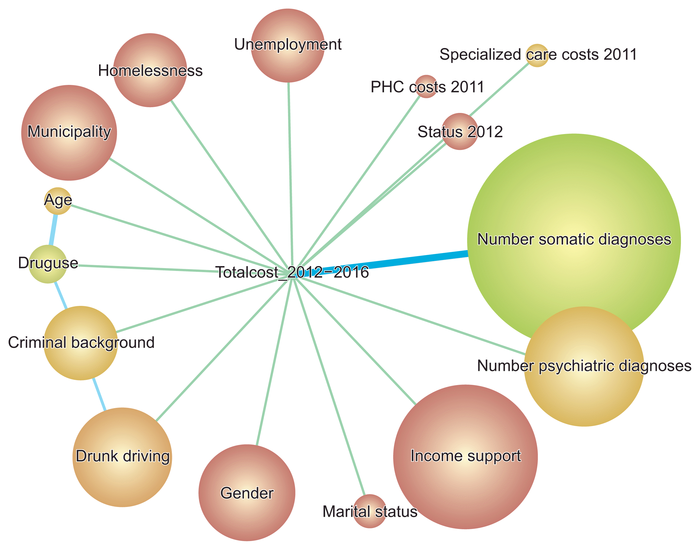
The ANB model is presented in Figure 2. The corresponding table of direct effects is Table 2, and the fixation table of the model is Tables 3 –5. The main finding was that a high number of somatic diagnoses was the strongest contributor to the 5-year total costs, causing over €26,000 mean excess cost per patient.

Figure 2

The augmented naive Bayes model of factors associated with the outcome variable total costs (totalcost_2012–2016). Node sizes express each variable’s direct effect on the target node. Node colors indicate node force, with green being the highest and red lowest, and yellow in between. Lines between nodes indicate the relationship between them (Kullback-Leibler divergence).

Table 2

Variables’ direct effects on and contributions to the target (totalcosts_2012–2016)

Variable	Direct effect on target (€)	Contribution (%)
Number of somatic diagnoses	26,345.44	37.5
Specialized care costs in 2011	1.10	13.6
Drunk driving	−12,896.21	11.1
Age	454.26	8.8
Income support	12,269.91	8.3
Gender	8,105.01	6.2
Unemployment	−5,668.21	4.6
Homelessness	−7,900.20	3.4
Primary health care costs in 2011	2.05	1.7
Municipality	−234.42	1.4
Drug use	1,465.75	1.2
Marital status	−1,038.56	0.7
Number of psychiatric diagnoses	553.47	0.6
Status in 2012	−326.87	0.3

The direct effect of each variable was calculated as the delta mean of the target variable when conditioning on maximum vs. minimum value of the variable one at a time, while others were fixed.

Table 3

Fixation table demonstrating values of the outcome variable (totalcosts_2012–2016) when the model is fixed to selected values (socio-economic variables)

Model#	Fixation	Quartile	Values of total costs of care (%)
1	No fixation	Q1	25.1
		Q2	25.1
		Q3	25.1
		Q4	24.7

4	Municipality, province capital = 100%	Q1	21.6
		Q2	23.9
		Q3	25.6
		Q4	29.0

5	Age, ≤35 yr = 100%	Q1	36.0
		Q2	23.0
		Q3	19.7
		Q4	21.3

6	Age, 36–45 yr = 100%	Q1	25.3
		Q2	28.2
		Q3	25.4
		Q4	21.1

7	Age, 46–55 yr =100%	Q1	20.7
		Q2	30.4
		Q3	28.2
		Q4	20.7

8	Age, ≥56 yr =100%	Q1	24.0
		Q2	16.7
		Q3	23.9
		Q4	35.4

9	Marital status 0 (single, divorced, widowed) = 100%	Q1	24.7
		Q2	25.1
		Q3	25.1
		Q4	25.1

10	Marital status 1 (married or cohabiting) = 100%	Q1	26.1
		Q2	25.0
		Q3	25.0
		Q4	23.9

11	Gender, male = 100%	Q1	26.9
		Q2	24.2
		Q3	26.5
		Q4	22.4

12	Gender, female = 100%	Q1	20.0
		Q2	27.4
		Q3	21.0
		Q4	31.6

Model 1 shows results of an unfixed model; Models 2–38 are done by fixing one separate value. Q1 and Q4 represents the lowest costs and highest costs, respectively.

Table 4

Fixation table demonstrating values of the outcome variable (totalcosts_2012–2016) when the model is fixed to selected values (clinical variables)

Model#	Fixation	Quartile	Values of total costs of care (%)
13	Status in 2012, Continuous drinking = 100%	Q1	23.6
		Q2	23.4
		Q3	26.3
		Q4	24.7

14	Status in 2012, Remission = 100%	Q1	42.9
		Q2	21.4
		Q3	10.7
		Q4	25.0

15	Number of somatic diagnoses, 0 (no diagnosis) = 100%	Q1	44.6
		Q2	38.5
		Q3	14.5
		Q4	2.4

16	Number of somatic diagnoses, 1 (one diagnosis) = 100%	Q1	37.2
		Q2	33.3
		Q3	21.8
		Q4	7.7

17	Number of somatic diagnoses, 2 (two or more diagnoses) = 100%	Q1	12.4
		Q2	16.3
		Q3	30.7
		Q4	40.6

18	Number of psychiatric diagnoses, 0 (no diagnosis) = 100%	Q1	28.2
		Q2	26.7
		Q3	24.2
		Q4	20.9

19	Number of psychiatric diagnoses, 1 (one diagnosis) = 100%	Q1	17.0
		Q2	17.0
		Q3	34.1
		Q4	31.9

20	Number of psychiatric diagnoses, 2 (two or more diagnoses) = 100%	Q1	12.8
		Q2	23.1
		Q3	20.5
		Q4	43.6

21	Specialized care costs in 2011, Q1 = 100%	Q1	30.7
		Q2	28.6
		Q3	19.8
		Q4	20.9

22	Specialized care costs in 2011, Q2 = 100%	Q1	28.6
		Q2	20.9
		Q3	26.3
		Q4	24.2

23	Specialized care costs in 2011, Q3 = 100%	Q1	24.2
		Q2	35.1
		Q3	26.4
		Q4	14.3

24	Specialized care costs in 2011, Q4 = 100%	Q1	16.7
		Q2	15.5
		Q3	27.8
		Q4	40.0

25	Primary health care costs in 2011, Q1 = 100%	Q1	29.5
		Q2	23.8
		Q3	22.9
		Q4	23.8

26	Primary health care costs in 2011, Q2 = 100%	Q1	24.7
		Q2	28.5
		Q3	20.8
		Q4	26.0

27	Primary health care costs in 2011, Q3 = 100%	Q1	24.2
		Q2	26.4
		Q3	26.4
		Q4	23.0

28	Primary health care costs in 2011, Q4 = 100%	Q1	21.1
		Q2	22.2
		Q3	30.0
		Q4	26.7

Model 1 shows results of an unfixed model; Models 2–38 are done by fixing one separate value. Q1 and Q4 represents the lowest costs and highest costs, respectively.

Table 5

Fixation table demonstrating values of the outcome variable (totalcosts_2012–2016) when the model is fixed to selected values (social deprivation variables)

Model#	Fixation	Quartile	Values of total costs of care (%)
29	Drunk driving, 0 (no) = 100%	Q1	24.7
		Q2	24.6
		Q3	24.0
		Q4	26.7

30	Drunk driving, 1 (yes) = 100%	Q1	26.8
		Q2	26.7
		Q3	29.6
		Q4	16.9

31	Income support, 0 (no) = 100%	Q1	39.1
		Q2	24.6
		Q3	21.8
		Q4	14.5

32	Income support, 1 (yes) = 100%	Q1	21.8
		Q2	25.2
		Q3	25.8
		Q4	27.2

33	Unemployment, 0 (no) = 100%	Q1	29.3
		Q2	17.2
		Q3	24.2
		Q4	29.3

34	Unemployment, 1 (yes) = 100%	Q1	23.1
		Q2	26.7
		Q3	25.5
		Q4	22.7

35	Drug use, 0 (no) = 100%	Q1	26.5
		Q2	24.8
		Q3	23.2
		Q4	25.5

36	Drug use, 1 (yes) = 100%	Q1	18.5
		Q2	26.2
		Q3	33.8
		Q4	21.5

37	Homelessness, 0 (no) = 100%	Q1	26.0
		Q2	24.6
		Q3	24.0
		Q4	25.4

38	Homelessness, 1 (yes) = 100%	Q1	12.0
		Q2	32.0
		Q3	40.0
		Q4	16.0

39	Criminal background, 0 (no) = 100%	Q1	25.6
		Q2	24.9
		Q3	25.9
		Q4	23.6

40	Criminal background, 1 (yes) = 100%	Q1	22.9
		Q2	25.7
		Q3	21.4
		Q4	30.0

Model 1 shows results of an unfixed model; Models 2–38 are done by fixing one separate value. Q1 and Q4 represents the lowest costs and highest costs, respectively.

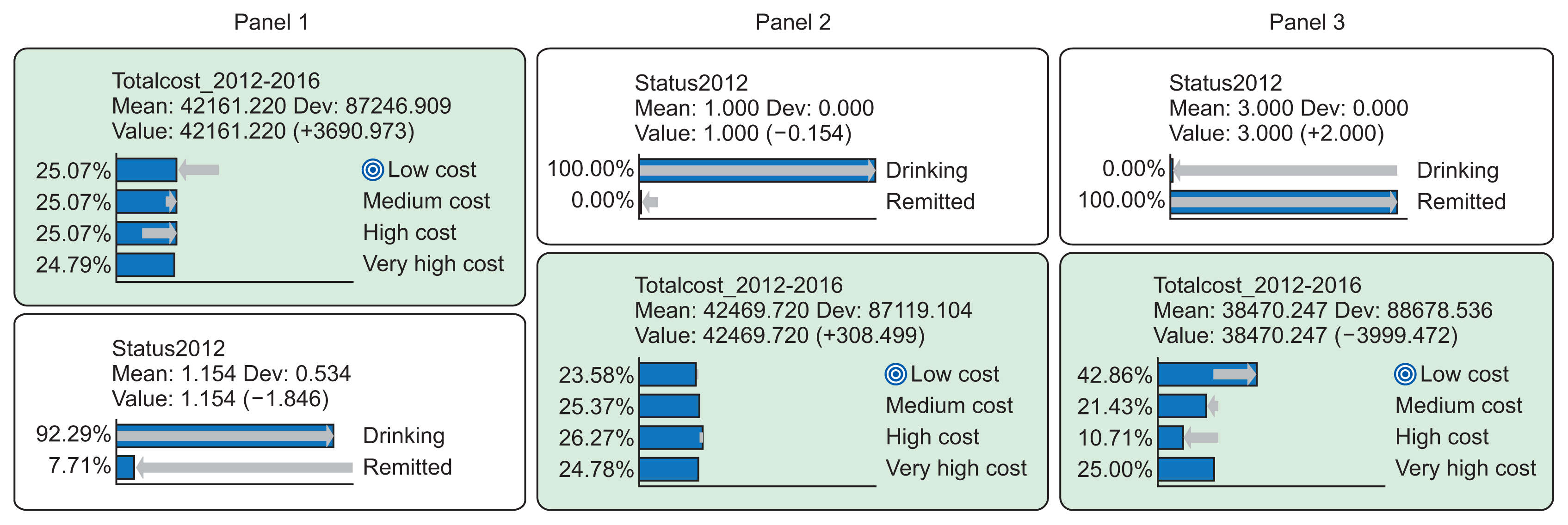
Secondly, the causal effect of an AUD remission was produced by fixing the variable “status2012” by turns to values 1 = continuous drinking and 3 = remitted. All other variables were controlled by fixing them to their original value distributions. The results presented in Figure 3 confirm our hypothesis that remission had a cost-decreasing effect on the cost accumulation, as the percentage of the lowest cost quartile was 42.86%, compared with the respective figure of 25.07% for current drinkers. Correspondingly, the percentage of the high-cost quartile was among remitters (10.71%) and among current drinkers (26.27%), while the proportion of very high costs remained on a rather similar level.

Figure 3

Panels showing the outcome variable “total cost_2012–2016” in relation to drinking “status2012”. Cost quartiles include: low costs, ≤€4,486.54; medium cost, €4,486.55–€15,746.10; high cost, €15,746.11–€46,864.36; and very high cost, €46,864.37–€1,180,863.75 and drinking status in 2012 was defined as continuous drinking versus remitted. In Panel 1, both variables are unfixed. Panel 2 shows the distribution of costs in the outcome variable “totalcost_2012–2016” when the variable “status2012” is fixed for the value drinking=100% and all other variables (not shown) are fixed to their original distribution. In Panel 3, the variable “status2012” is fixed for the value remitted=100%, demonstrating the causal change in costs (totalcost_2012–2016) after achieving remission.

Comparative SAs with tornado diagrams are presented in Figure 4. The diagrams show that the number of somatic diseases, specialized care costs, number of psychiatric diagnoses, age, and drug use have the strongest impact on high and very high costs of care. SAs of values that (1) maximize the costs and (2) minimize the costs during the 5-year follow-up are presented in Tables 6 and 7. These profiles strongly suggest that the excess costs of AUD patients are caused by multimorbidity. Joint probability values less than 1 (in both Tables 6 and 7) indicate the results in this cohort, but we consider them ungeneralizable outside this cohort.

Figure 4

Tornado diagrams showing variables with the strongest impact on the outcome variable. Bars pointing to the right represent a positive impact, and bars to the left a negative impact. (A) Panel 1 shows the effect on “low cost” value of the outcome variable, (B) Panel 2 on “medium cost”, (C) Panel 3 on “high cost”, and (D) Panel 4 on “very high cost”.

Table 6

Dynamic profile of values maximizing the outcome variable total 5-year cost (totalcosts_2012–2016)

Node	Optimal state	Value/mean	95% credible interval	Joint probability (%)
A priori		42,161	5,315	100
Number of somatic diagnoses	2+	60,782	575	23.4
Specialized care costs in 2011	>4,588	78,479	5,733	5.3
Income support	Yes	81,799	5,668	5.4
Drunk driving	No	85,528	5,615	4.4
Municipality	Region capital	90,348	5,471	2.6
Gender	Female	98,883	5,160	0.8
Unemployment	No	104,284	4,849	0.3
Age	>55	114,029	4,046	0.04
Criminal background	Yes	120,624	3,263	0.02
Drug use	Yes	127,284	1,892	>0.00
Homelessness	No	127,607	1,803	>0.00
Number of psychiatric diagnoses	2+	128,804	1,416	>0.00
Primary health care costs in 2011	≤130	129,191	1,264	>0.00
Status in 2012	Stable remission	130,042	829	>0.00
Marital status	Single, divorced, or widowed	130,049	825	>0.00

Table 7

Dynamic profile of values minimizing the outcome variable total 5-year costs (totalcosts_2012–2016)

Node	Optimal state	Value/mean	95% credible interval	Joint probability (%)
A priori		42,161	5,315	100
Number of somatic diagnoses	No	12,711	23	8.1
Specialized care costs in 2011	≤191	10,418	1,958	2.6
Income support	No	7,602	1,434	0.5
Age	≤35	5,454	1,199	0.09
Municipality	Other	5,015	1,063	0.06
Homelessness	No	4,836	1,055	0.08
Gender	Male	4,621	991	0.07
Unemployment	No	411	1,008	0.03
Primary health care costs in 2011	≤27.4	3,691	917	0.01
Status in 2012	Stable remission	271	683	>0.00
Drug use	No	2,601	671	>0.00
Criminal background	No	2,565	639	>0.00
Drunk driving	Yes	2,505	530	>0.00
Marital status	Married or cohabiting	2,474	512	>0.00

Go to :

IV. Discussion

This is the first time that causality between multiple risk factors and cumulative healthcare costs among AUD patients was studied by using EHR data with the application of van der Weele and Shiptser’s modified DCC [24]. As the etiology and clinical course of AUD are complex and affected by numerous variables, a true causal network between the variables and the outcome variable remain unknown. In this study, causality was estimated by using the modified DCC to calculate the direct causal effect of individual variables on the cumulative healthcare costs from a non-causal Bayesian network. The results suggest that multiple chronic conditions together with high specialized care costs, receiving income support, region capital as a place of residence, and age over 55 years fulfilled the DCC and were the strongest explanatory factors maximizing the 5-year total costs. Respectively, the prevalence of the lowest cost quartile increased notably among those who remitted.

The clearest causal relationship was observed between the number of chronic conditions and the total costs of care. The SA of values maximizing the total cost of care identified a high number of chronic conditions to be the main contributor to the excess cost of care in this cohort and to increase the mean total cost by €26,000 per patient. Furthermore, SA with tornado diagrams showed that the variables that had the strongest impact on the total cost of care varied; for low cost value (<€4,486) of the target interval, the number of chronic conditions and baseline drinking status (status2012) had the strongest role. For the high (≤€46,864) and very high cost value (>€46,864.4) of the target interval, the role of comorbidity, social problems such as illicit drug use and homelessness, specialized care costs, psychiatric comorbidity, and age had the strongest impact.

However, there were certain limitations, and they should be considered when interpreting the findings. First, the cohort was formed retrospectively, and then follow-up was managed prospectively. We consider this method better than a completely retrospective method. Also, follow-up data from 33 individuals were missing (8.3%). Second, the DCC is used in situations in which the exact causal relations between variables are unknown. In this study, we were able to recognize only a few clear causal relations, such as the effect of multiple diseases, to increasing costs. Causalities between independent variables remained mostly unknown. The use of the DCC has two requirements. All independent variables should be known in pre-treatment condition, in this study, before the year 2012. Only variables fulfilling this criterion were used in this DCC analysis. The other requirement is that any unmeasured variable should have no effect on the index variable (status2012), the outcome, or both. For example, the genetic basis of AUD and motivation to adhere to treatment are potential unmeasured variables with an effect on AUD remission and costs. We consider these unmeasured variables as parent variables to the measured ones, and with regard to the motivation, status in 2012 is thought to function as a marker condition for motivation. However, we cannot rule out the potential bias generated by unmeasured variables. Third, the direct effect on the outcome variable shown in Table 2 requires that the impact of independent variables should be linear. However, some variables show an increasing nonlinear association with the outcome in the highest values. This was seen in the following variables: age, number of psychiatric diagnoses, and drug use. We consider that the direct effect analysis showed in Table 2 moderately underestimates their impact.

Although the results cannot be directly compared with those of previous studies due to differences in the study design and methodologies used, our findings support the previous evidence regarding the cost-decreasing effect of AUD remission [12,13]. Application of the DCC to study patients with AUD provided evidence that achieving stable remission decreased the total cost of care during the 5-year follow-up. Likewise, previous studies have indicated that high prevalence of comorbidities explains the increases in cost accumulation, especially among high-cost patients [22], which include patients with addictions [28]. Thus, our results are in line with those of previous studies identifying an association between the number of comorbidities and increased costs of care among patients with chronic conditions [22,29,30]. This research identified factors that minimize and maximize the total cost among AUD patients. The information provided by this study, especially regarding the cost-offset pattern of achieving AUD remission, supports decision-making in both clinical settings and at the policy level.

Go to :

Acknowledgments

This manuscript is a component of a PhD thesis for Elina Rautiainen at the University of Eastern Finland, who was supported by the Finnish Foundation for Alcohol Studies, and the University of Eastern Finland Graduate School. This study received funding from the Strategic Research Council at the Academy of Finland (No. 312703).

Go to :

Notes

Conflict of Interest

No potential conflict of interest relevant to this article was reported.

Go to :

References

1. Dennis M, Scott CK. Managing addiction as a chronic condition. Addict Sci Clin Pract. 2007; 4(1):45–55.

2. Witkiewitz K, Marlatt GA. Modeling the complexity of post-treatment drinking: it’s a rocky road to relapse. Clin Psychol Rev. 2007; 27(6):724–38.

3. National Institute on Alcohol Abuse and Alcoholism. Alcohol facts and statistics [Internet]. Bethesda (MD): National Institute on Alcohol Abuse and Alcoholism;c2019. [cited at 2020 Apr 1]. Available from: https://www.niaaa.nih.gov/publications/brochures-and-factsheets/alcohol-facts-and-statistics.

4. Effertz T, Mann K. The burden and cost of disorders of the brain in Europe with the inclusion of harmful alcohol use and nicotine addiction. Eur Neuropsychopharmacol. 2013; 23(7):742–8.

5. Gustavsson A, Svensson M, Jacobi F, Allgulander C, Alonso J, Beghi E, et al. Cost of disorders of the brain in Europe 2010. Eur Neuropsychopharmacol. 2011; 21(10):718–79.

6. Boschloo L, Vogelzangs N, van den Brink W, Smit JH, Beekman AT, Penninx BW. Predictors of the 2-year recurrence and persistence of alcohol dependence. Addiction. 2012; 107(9):1639–40.

7. Vaillant GE, Hiller-Sturmhofel S. The natural history of alcoholism. Alcohol Health Res World. 1996; 20(3):152–61.

8. Collins SE. Associations between socioeconomic factors and alcohol outcomes. Alcohol Res. 2016; 38(1):83–94.

9. Compton WM, Gfroerer J, Conway KP, Finger MS. Unemployment and substance outcomes in the United States 2002–2010. Drug Alcohol Depend. 2014; 142:350–3.

10. Cross GM, Morgan CW, Mooney AJ 3rd, Martin CA, Rafter JA. Alcoholism treatment: a ten-year follow-up study. Alcohol Clin Exp Res. 1990; 14(2):169–73.

11. Dennis ML, Foss MA, Scott CK. An eight-year perspective on the relationship between the duration of abstinence and other aspects of recovery. Eval Rev. 2007; 31(6):585–612.

12. Holder HD, Blose JO. The reduction of health care costs associated with alcoholism treatment: a 14-year longitudinal study. J Stud Alcohol. 1992; 53(4):293–302.

13. Zywiak WH, Hoffmann NG, Stout RL, Hagberg S, Floyd AS, DeHart SS. Substance abuse treatment cost offsets vary with gender, age, and abstinence likelihood. J Health Care Finance. 1999; 26(1):33–9.

14. Parthasarathy S, Weisner CM. Five-year trajectories of health care utilization and cost in a drug and alcohol treatment sample. Drug Alcohol Depend. 2005; 80(2):231–40.

15. Hoff RA, Rosenheck RA. The cost of treating substance abuse patients with and without comorbid psychiatric disorders. Psychiatr Serv. 1999; 50(10):1309–15.

16. Davenport T, Kalakota R. The potential for artificial intelligence in healthcare. Future Healthc J. 2019; 6(2):94–8.

17. Escobar GJ, Turk BJ, Ragins A, Ha J, Hoberman B, LeVine SM, et al. Piloting electronic medical record-based early detection of inpatient deterioration in community hospitals. J Hosp Med. 2016; 11(Suppl 1):S18–S24.

18. Liang H, Tsui BY, Ni H, Valentim CC, Baxter SL, Liu G, et al. Evaluation and accurate diagnoses of pediatric diseases using artificial intelligence. Nat Med. 2019; 25(3):433–8.

19. Abhari S, Niakan Kalhori SR, Ebrahimi M, Hasannejadasl H, Garavand A. Artificial intelligence applications in type 2 diabetes mellitus care: focus on machine learning methods. Healthc Inform Res. 2019; 25(4):248–61.

20. Morid MA, Kawamoto K, Ault T, Dorius J, Abdelrahman S. Supervised learning methods for predicting healthcare costs: systematic literature review and empirical evaluation. AMIA Annu Symp Proc. 2018; 2017:1312–21.

21. Yang C, Delcher C, Shenkman E, Ranka S. Machine learning approaches for predicting high cost high need patient expenditures in health care. Biomed Eng Online. 2018; 17(Suppl 1):131.

22. Wammes JJ, van der Wees PJ, Tanke MA, Westert GP, Jeurissen PP. Systematic review of high-cost patients’ characteristics and healthcare utilisation. BMJ Open. 2018; 8(9):e023113.

23. BayesiaLab [Internet]. Franklin (TN): Bayesia USA;2019. [cited at 2020 Apr 1]. Available from: http://www.bayesialab.com/.

24. Rissanen J. Modeling by shortest data description. Automatica. 1978; 14:465–71.

25. VanderWeele TJ, Shpitser I. A new criterion for confounder selection. Biometrics. 2011; 67(4):1406–13.

26. VanderWeele TJ. Principles of confounder selection. Eur J Epidemiol. 2019; 34(3):211–9.

27. Conrady L, Jouffe L. Bayesian networks and BayesiaLab: a practical introduction for researchers. Franklin (TN): Bayesia USA;2015.

28. Hensel JM, Taylor VH, Fung K, Vigod SN. Rates of mental illness and addiction among high-cost users of medical services in Ontario. Can J Psychiatry. 2016; 61(6):358–66.

29. Shei A, Rice JB, Kirson NY, Bodnar K, Enloe CJ, Birnbaum HG, et al. Characteristics of high-cost patients diagnosed with opioid abuse. J Manag Care Spec Pharm. 2015; 21(10):902–12.

30. Lahiri B, Agarwal N. Predicting healthcare expenditure increase for an individual from medicare data. In : Proceedings of the ACM SIGKDD Workshop on Health Informatics; 2014 Aug 24; New York City, NY.

Go to :

Appendices

Appendix 1

Alcohol-related ICD-10 codes used in sampling

ICD-10 code	Label
G31.2	Degeneration of nervous system due to alcohol
G40.5	Special epileptic syndromes
G40.50	Epilepsia partialis continua [Kozhevnikof]
G40.51	Epileptic seizures related to alcohol
G40.52	Epileptic seizures related to drugs
G31.2	Degeneration of nervous system due to alcohol
G62.1	Alcoholic polyneuropathy
I42.6	Alcoholic cardiomyopathy
K29.2	Alcoholic gastritis
F10	Mental and behavioral disorders due to psychoactive substance use
F10.0	Acute intoxication
F10.1	Harmful use
F10.2	Dependence syndrome
F10.3	Withdrawal state
F10.4	Withdrawal state with delirium
F10.5	Psychotic disorder
F10.6	Amnesic syndrome
F10.8	Other mental and behavioral disorders
F10.9	Unspecified mental and behavioral disorder
K86.0	Alcohol-induced chronic pancreatitis
K70.0	Alcoholic fatty liver
K70.1	Alcoholic hepatitis
K70.2	Alcoholic fibrosis and sclerosis of liver
K70.3	Alcoholic cirrhosis of liver
K70.4	Alcoholic hepatic failure
K70.9	Alcoholic liver disease, unspecified
T51	Toxic effect of alcohol
T51.0	Ethanol
T51.1	Methanol
T51.2	2-Propanol
T51.3	Fusel oil
T51.8	Other alcohols
T51.9	Alcohol, unspecified
X45	Accidental poisoning by and exposure to alcohol
X69	Intentional self-poisoning by and exposure to other and unspecified chemicals and noxious substances

ICD-10: the 10th revision of the International Statistical Classification of Diseases and Related Health Problems.

Appendix 2

Costing methodology

In this study, patient-level cost data was directly available from two linked EHR (Electronic Health Record) systems. Direct costs from specialized care were retrieved from the central hospital’s cost accounting systems for the years 2011 to 2016 including all hospitalizations, outpatient costs, and admissions. Direct costs from primary care were retrieved from municipal EHRs, which include patient-level costs. Overall, the accuracy and coverage of the publicly funded social and healthcare services’ cost accounting data are considered reliable, especially regarding expensive treatments. North Karelia is a sparsely populated region with only a few private social and healthcare providers; thus the coverage of the public data sources is considered comprehensive. However, it should be noted that cost data regarding private healthcare was lacking from the primary care EHR registers.

Appendix 3

Mathematical formula of minimum description length (MDL) score

$MDL (BN, Data) = - \sum_{j = 1}^{N} log 2 (P_{B} (e_{j})) + SC * (\sum_{i = 1}^{n} (log 2 (n) + {log}_{2} (\begin{matrix} n \\ ‖ π i ‖ \end{matrix})) + \sum_{i = 1}^{n} (\prod_{j = 1}^{‖ π i ‖} S j * (S i - 1) * {log}_{2} (N) / 2),$

where e_j is the n-dimensional observation of the row j, P_B is the joint probability of this observation from the Bayesian network, n is the number of random variables, X_i ||πi|| is the number of parents of a variable X_i, and Si is the number of states of random variable X_i. [29].

Go to :

TOOLS

Similar articles