Microscopic analysis of hematoxylin and eosin (H&E) stained tissue slides has been the basis for disease diagnosis for decades [1]. The diagnosis is based on a visual interpretation of tissue structures and other pathological tissue characteristics by human interpreters. However, many studies have shown inconsistencies in diagnostic decisions, leading to poor reproducibility [23]. Because the interpretation of tissue morphology is often subjective, both intra- and inter-observer variations are frequent and can lead to misdiagnosis [4]. Thus, many cancer centers encourage consensus between multiple observers on oncologic diagnoses [5]. Although it is optimal for a slide to be reviewed by multiple experts, it is usually very costly and may delay the final decision because the histological assessment of tissue slides is time-consuming and laborious. Considering the shortage of pathologists in hospitals, routine peer-review of tissue slides may be impractical. Thus, machine learning-based analysis of tissue slides has been studied for decades to complement human decisions [67].

Machine learning is a method of creating a task-specific computational model from a given dataset [8]. Typically, it requires domain-specific features to be extracted from raw data based on the knowledge of domain experts, followed by statistical modeling and learning steps based on these extracted features. Thus, it requires considerable domain expertise and complex feature selection steps. In contrast, feature extraction and model learning take place in a unified step in deep learning [9]. Deep learning-based approaches have become very successful in a wide range of biomedical analysis tasks [10], including the analysis of retinal fundus images [11], radiologic images [12], pathologic tissue images [13], electrocardiograms [14] and electroencephalograms [15]. However, deep learning-based methods generally require large annotated datasets compared to traditional machine learning [16]. The recent introduction of digitization of whole slide images (WSIs) using slide scanners has provided large amounts of digital histopathology data for the application of deep learning [6]. Accordingly, considerable efforts have been made to utilize deep learning for the analysis of WSIs [8].

One of the basics of histopathology image analysis is the classification of tissue slides into normal or diseased tissues, an important step in the development of computer-aided diagnosis (CAD) systems. In the present study, we developed deep learning-based, fully automated classifiers for WSIs of normal/tumor stomach tissues obtained from The Cancer Genome Atlas (TCGA) [17]. WSIs inevitably contain out-of-focus/blurry areas because the autofocusing capability of whole slide scanners are not yet perfect. In addition, there are various artifacts, including air-bubbles, compression artifacts, over- or under-staining, pen markings, and tissue folding [18]. To construct a fully automated classification process, these artifacts should be automatically removed. Thus, we first constructed a classifier that selected proper tissue regions. The selected tissue regions were then classified into normal or tumor regions by another classifier. Since no single network structure can solve all medical imaging problems [19], we tested three different convolutional neural networks (CNNs) to see whether specific network structures were more suitable for the analysis of histopathology images. When we applied this two-step approach for slide level classification, it clearly demonstrated that a deep learning-based approach can be used to build a fully automated CAD system for frozen tissue slides in the near future. Finally, we validated the classifier with our own dataset to assess the generalizability of the model generated with the TCGA dataset.

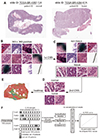
The TCGA program provides extensive archives of digital pathology slides. The provided WSIs are composed of frozen section tissue slides and formalin-fixed paraffin-embedded diagnostic slides. The frozen sections directly relate to tissue regions where multi-omics information in the TCGA program was analyzed, making them more relevant for studies of the relationship between histomorphology and molecular profiles [17]. Thus, in this study, we built a deep learning-based classifier for normal/tumor tissues from the frozen tissue slides of stomach adenocarcinoma (TCGA-STAD). Informed consent was obtained by the TCGA consortium [2021] and all WSIs were publicly available for research purposes. Accordingly, institutional review board approval was not required. There were 755 tissue slides in TCGA-STAD, and we omitted 2 slides because of suboptimal quality. Consequently, a total of 753 slides from 432 patients were included in the present study. There were 122 normal tissue slides and 631 tumor slides. These normal or tumor tissues slides consisted of almost exclusive normal or tumor tissues which were confirmed by the reviewing pathologists of TCGA consortium (Fig. 1A).

Since WSIs are too big to be analyzed by CNNs at once, we segmented the WSIs into non-overlapping 360 × 360 pixels patches at 20× magnification (resultant pixel resolution of 0.24 µm/pixel). Total patch numbers from a WSI ranged from hundreds to thousands depending on the size of the WSI. Labels for the patches were automatically obtained from the identifiers (IDs) of the WSIs (Fig. 1A). Every patch in a WSI was labeled as either normal or tumor based on the slide ID because each tissue slide was almost exclusively composed of either normal or tumor stomach tissue.

After initial segmentation, there were huge amount of improper patches, including air-bubbles, compression artifacts, pen markings, tissue folding, and white background, all of which required elimination before classification of normal and tumor tissue. Preprocessing such as Otsu thresholding can be used to eliminate white background. However, we tried to remove the improper patches all at once. Thus, we constructed a simple first CNN with three convolutional-pooling layers to classify tissue/non-tissue patches. The three convolution layers consisted of 12 [5 × 5] filters, 24 [5 × 5] filters and 24 [5 × 5] filters, each followed by a [2 × 2] max-pooling layer. To train the CNN, S.H.L. collected 10,000 improper and 10,000 proper tissue patches and trained the CNN to distinguish patches into non-tissue and tissue, respectively (Fig. 1B, C). Only patches classified as tissue were used for the next step. For normal/tumor classification, we implemented three well-known CNN architectures, AlexNet, ResNet-50 and Inception-v3, which showed good performance in a natural image classification contest [22]. The three CNN architectures were trained to distinguish selected tissue patches into normal or tumor patches (Fig. 1C, D).

We adopted ten-fold cross validation to validate the functionality of the classifiers. In the ten-fold cross validation scheme, ten exclusive combinations of training/test sets were composed in which one tenth of the data are allocated to test sets and the rest to training sets. In all folds, training and test sets were split on a patient level and no tissue slides from the training patients were present in the test set. The results from each fold were concatenated to assess the total classification results.

Data augmentation was applied during training to promote learning of most robust general features for distinguishing between normal and tumor tissue. We performed random cropping of 330 × 330 regions from the 360 × 360 patches, followed by random rotations by 90°, random horizontal/vertical flipping, and random transformations of contrast and brightness. We used mini-batches of size 128 for training. The TCGA-STAD tissue slides had an innate class imbalance problem because there were more than four times fewer normal patches than tumor patches. The average numbers of normal and tumor patches for the training set in each fold were 318,631 and 1,440,396, respectively. To alleviate the deteriorative effect of the class imbalance, we supplied the same number of normal and tumor patches in a minibatch. Since we used a mini-batch size of 128, 64 normal and 64 tumor patches were used for each mini-batch. As another approach to alleviate the class imbalance, we tested weighted cross entropy loss function which gives more weight to loss component for samples from under-represented class. The output layer used a softmax activation function for two nodes to compute an output probability distribution over normal and tumor tissue before the cross entropy loss function. All the CNN networks were implemented using the Tensorflow library (http://tensorflow.org).

The widely-used classification evaluation criteria including accuracy, sensitivity, specificity, and area under the curve (AUC) for receiver operating characteristic (ROC) curves are presented in this study. Accuracy, sensitivity and specificity were calculated with the threshold for normal/tumor discrimination set to 0.5. ROC curves plot the true positive (sensitivity) versus the false positive (1-specificity) fraction by adjusting the threshold for normal/tumor discrimination, allowing sensitivity and specificity tradeoffs to be evaluated [23]. In this study, to calculate the sensitivity and specificity, tumor tissue was considered positive and normal tissue negative. To compare differences between the two ROC curves, we applied a permutation test with 1,000 iterations [24]. After analyzing classification performance at the patch level, we investigated classification performance at the slide level. To do this, the probability for each slide was calculated as the average of the probabilities of all the patches in the slide. Averaging of patchlevel classification results can be applied to assess the slide-level classification because the TCGA-STAD tissue slides were almost exclusively composed of either normal or tumor stomach tissue. Based on the average value, slide-level ROCs were plotted. A p-value < 0.05 was considered significant.

To validate the model obtained from TCGA-STAD dataset, we built an extra validation dataset of frozen tissue slides obtained during surgical procedures in the Seoul St. Mary's Hospital. Tissue collection were conducted in accordance with protocols approved by the Institutional Review Board of The Catholic University of Korea (KC19SESI0787). The dataset consisted of 25 normal and 25 tumor slides. The slides which consisted of almost exclusive normal or tumor tissues were carefully selected by S.H.L., who has been a specialist for gastrointestinal pathology in the Seoul St. Mary's Hospital for more than 5 years. We named the dataset as SSMH-STAD. At first, whole 50 slides were classified with network trained with TCGA-STAD. Next, 5 slides of SSMH-STAD from each class were co-trained with TCGA-STAD dataset. Because SSMH-STAD data in the new training set was more than fifteen times fewer than TCGA-STAD data, SSMH-STAD could be severely underrepresented when mini-batch was randomly selected from total training data. Thus, in the cotraining scenario, 30% of data in a mini-batch was intentionally selected from SSMH-STAD to promote the learning of features in the SSMH-STAD dataset.

To make the classification of tissue slides fully automated, white background regions and artifacts should be automatically excluded from further processing. In this study, we implemented a simple CNN to delineate improper patches regardless of whether they were background or artifacts (Fig. 1B). When we applied the simple CNN for non-tissue/tissue classification, the accuracy was more than 98% compared to human annotation. Because the classification of improper tissues is a relatively subjective issue, we decided that 98% was sufficient to proceed. Next, we trained AlexNet, ResNet-50 and Inception-v3 to distinguish the tissue patches into normal or tumor to compare the performance of different CNN architectures. For each fold, we first obtained classification results on the test patches of the corresponding folds and then concatenated all the results from the ten folds to calculate accuracy, sensitivity and specificity. ROCs were also plotted on the concatenated results.

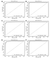
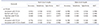
The classification results for the three architectures are summarized in the upper part of Table 1. The patch-level classification results for Inception-v3 (Fig. 2A) was better than ResNet-50 (Fig. 2C) and AlexNet (Fig. 2E) (p < 0.001 by permutation test). Since slide level labels were originally assigned to the WSIs, slide-level classification results could easily be compared with the labels. We obtained slide level probabilities by averaging patch level classification probabilities. ROC curve for the slide-level classification did not differ by permutation test between Inception-v3 (Fig. 2B), ResNet-50 (Fig. 2D) and AlexNet (Fig. 2F). When cut-off value for normal/tumor discrimination was set at 0.5, they all shared 6 normal tissues falsely classified as tumor. However, the number of tumor tissues falsely classified as normal was different as 3, 4 and 7 for Inception-v3, ResNet-50 and AlexNet, respectively. Based on the patch- and slide-level classification results, we concluded that Inception-v3 is the most suitable CNN structure for stomach tissue classification between the three CNNs.

Because there were more than four times tumor tissues than normal tissues in the TCGA-STAD dataset, we implemented balanced mini-batch approach to alleviate the class imbalance problem. However, the sensitivity was still higher than the specificity for all three CNN architectures (Table 1). As another approach, weighted cross entropy approach was tested with Incetion-v3. We gave ten times more weight to the loss for the normal class. In this case, the specificity was improved from 0.920 to 0.932 but the sensitivity was decreased from 0.958 to 0.951, resulting overall decrease in the accuracy from 0.953 to 0.947. As the last approach, we randomly selected one fourth of the tumor training data to match the number of normal and tumor data. This approach yielded best specificity of 0.942, but sensitivity and accuracy were also decreased to 0.941 and 0.941, respectively. Thus, specificity can only be improved with the decrease in the sensitivity and accuracy. The patch- and slide-level classification results in Fig. 2 were all obtained with the balanced mini-batch approach which yielded the best overall accuracy.

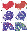
Next, we overlaid the patch level classification results of Inception-v3 on the tissue images of WSIs to depict the distribution of normal/tumor tissue regions in the slides (Fig. 3). Either binary normal/tumor maps (Fig. 3, left panels, blue for normal and red for tumor patches) or probability heatmaps (Fig. 3, right panels, color gradient changing from blue to red with increased probability of tumor) were drawn for comparison. Through this mapping, we identified three categories of tissues. The first was clear tumor cases, which contained huge aggregated red regions in the tissue map (Fig. 3A). The second was clear normal cases, which only contained a few dispersed red or green spots without aggregation (Fig. 3B). The last was ambiguous cases with lots of aggregated red or green spots (Fig. 3C). Thus, tissue properties could be easily determined by the mapping.

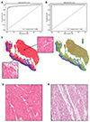
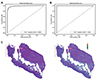
Finally, we validated the Inception-v3 model trained on TCGA-STAD with our own frozen tissue dataset named SSMH-STAD (Fig. 4). The patch-level classification result on SSMH-STAD was inferior to the classification results for the TCGA-STAD test set (Fig. 4A). Although ROC curve for slide-level classification showed perfect curve with AUC of 1.000 (Fig. 4B), there were 11 normal tissues falsely classified as tumor when the cut-off threshold for normal/tumor discrimination was set to 0.5. The results indicated that normal and tumor slide can be clearly demarcated by a certain cut-off threshold point other than 0.5. The deviation was thought to be originated from the poor classification results on normal tissues because specificity was much lower than sensitivity in both patch- and slide-levels (lower part of Table 1). Thus, we reviewed the heatmaps of misclassified tissues to clarify the reason of poor classification results for normal tissues. We found that most misclassified parts of normal tissues were muscle structures (Fig. 4C). When we compared the muscle tissues in the SSMH-STAD (Fig. 4D) and the TCGA-STAD (Fig. 4E), we concluded that the preparation quality was very different. Although the muscles in the SSMH-STAD were very densely packed and clearly demonstrated their natural structural patterns, muscles in TCGA-STAD showed loose degraded patterns. To test if the different features of the SSMH-STAD dataset can be incorporated into the neural network by exposing a small amount of the SSMH-STAD data into the original TCGA-STAD training data, we appended 5 normal and 5 tumor slides from the SSMH-STAD into the TCGA-STAD training data for fold 1 of the ten-fold cross validation set of the TCGA-STAD. Thus, we performed five-fold cross validation on the SSMH-STAD dataset with the fold 1 of TCGA-STAD dataset. Because the numbers of the SSMH-STAD data were much fewer than the TCGA-STAD data, we trained the neural network with mini-batches containing 30% of the SSMH-STAD data to promote the learning of the features unique to the SSMH-STAD dataset. The results for patch-level classification was greatly improved (Fig. 5A, p < 0.001 by permutation test). Furthermore, there were no falsely classified slides even with the cut-off threshold of 0.5 in this setting. This improvement did not ameliorate the classification performance on the TCGA-STAD test data for fold 1 (data not shown). Thus, by supplying a small amount of the SSMH-STAD data, we could construct a classifier for both datasets.

The purpose of this study was to develop a deep learning-based, fully-automated classifier for WSIs. With the classifier, we tried to explore the possibilities of a decision support system which can assist with laborious tissue analysis tasks. Among the many architectures of deep learning, CNN has become the standard for image classification problems because it outperforms other machine learning methods for various image recognition tasks by learning spatially invariant features directly from huge image databases [2526]. Thus, we adopted CNNs for the automated classifier of tissue slides in the current study.

For automated processing, artifacts and background must be eliminated, because these images contain information completely irrelevant for the main tasks of normal/tumor tissue discrimination. Irrelevant images can deteriorate the learning process of deep neural networks. To exclude white background, many researchers have adopted the Otsu thresholding algorithm [1827]. A recent study by Senaras et al. [18] was completely dedicated to the removal of out-of-focus images. We used a much simpler CNN, but achieved acceptable performance for the removal of not only out-of-focus images but also all the other irrelevant images, including air-bubbles, compression artifacts, pen markings, tissue folding and white background. Thus, we concisely solved the issue of irrelevant tissue removal with a simple CNN.

In general, deep learning requires huge amounts of data for training. Recently, routine digitization of tissue slides has started to supply plenty of data for the application of deep learning to a wide variety of applications. Because the US Food and Drug Administration approved the use of WSIs for primary diagnostic use, efforts to apply computerized analysis to WSIs are expected to explode in the near future [16]. One of the most imminent applications will be in CAD systems that complement human diagnosis. Because diagnostic decisions based on histopathology have shown inter- and intra-observer variability [23], CAD systems offer increased efficiency and accuracy.

When we first designed the experiment, we expected the performance of the three CNN structures to be very different, because they showed substantially different performances in the ImageNet Large Scale Visual Recognition Challenge (ILSVRC) [22]. However, the difference was much smaller than expected, although the order of performance was the same as that obtained from the ILSVRC, i.e., the performance got better in the order of AlexNet, ResNet-50 and Inception-v3. The ILSVRC contained about 1,000 to 1,500 image samples per class for a thousand classes. In contrast, many more image samples for just two classes were classified in the current experiment. We speculate that the innate potential of the three CNN structures as classifiers of images does not differ much when plenty of image samples can be supplied. However, when samples are limited, performance gaps can widen. Otherwise, features for the classification of tissue images can be quite different from natural images because there are relatively simple repetitive patterns in histologic images. Additional considerations in the selection of network structures include computational load and memory requirements, which differ between the CNN structures. Thus, network structures should be selected depending on the nature of the images, sample sizes, number of total classes and available computing power.

Another important subject to address is the class imbalance problem. In the TCGA-STAD tissue slide dataset, considerably fewer normal slides were provided than tumor slides. Ideally, deep learning requires a similar amount of training data between the classes. If there is a large imbalance between the classes, the deep learning model cannot fully learn the characteristics of under-represented classes [19]. One of the methods for alleviating the class imbalance problem is to sample the same amount of training data from each class [28]. However, if this method is applied by random sampling, it inevitably omits some information from the majority class. To avoid this, more informative samples should be carefully selected. This is a very difficult task, especially for a huge amount of tissue image patches. Thus, we chose to apply the balanced mini-batch method at first. By supplying the same number of data for each class in the mini-batch, preference for the majority class could be alleviated. Although we applied this method, the sensitivity was much higher, i.e., the CNNs still classified tumor patches more correctly. When we applied the weighted cross entropy loss function, the specificity was slightly improved but accompanied by the decrease in the accuracy and sensitivity. The best method to improve the specificity was the subsampling method for the tumor training data. In this case, the accuracy and sensitivity became much worse. These results indicated that there is an innate limitation to solve the class imbalance problem through sampling methods or modified loss function. The best solution is to build a balanced dataset from the beginning, if possible.

The purpose of a CAD system is to improve the efficiency, accuracy, and consistency of the diagnostic process, particularly in a time-limited clinical setting. The system can improve the age-old problem of inter-observer variation, leading to much better clinical outcomes for patients. By drawing heatmaps overlaid on the WSIs, we tested the potential of our system for these objectives. There were three distinguishable categories of clear normal, clear tumor and ambiguous cases (Fig. 3). If heatmaps are provided before inspection by human interpreters, the clear normal cases can be put aside and more time can be given to the ambiguous cases. By automatically screening for cases that require more attention, this system can guide the pathologists to arrange their time and efforts during the routine diagnostic process. Alternately, the system can be applied after manual inspection as part of a pathology laboratory's quality management process.

Another application of these heatmaps is confirmation of the boundary of tumor regions. Recently, a lot of omics information, including genomics, transcriptomics, and proteomics, has been integrated into the diagnostic and prognostic evaluation of disease [5]. Such molecular examination of solid tumor tissue often requires the percentage of tumor tissue as a fraction of the entire sample. However, assessing this visually can be highly subjective and poorly reproducible [29]. Heatmaps can provide clear quantitative and spatial distribution information about the tumor in the tissue. In addition, they can assist with the automated sectioning of tumor regions for relevant multi-omics testing from the beginning. This approach can improve the confidence of molecular tests, because clear tumor regions can be used for the tests in both clinical and experimental settings.

One limitation of the TCGA-STAD dataset is that it consists of mainly Caucasian patients and collected from the hospitals in the United States. Ethnicity is thought to be an important factor that determines the characteristics of tumor tissues. Thus, a classifier trained on Caucasian tissues does not show the same performance on tissues of Asian patients [30]. It has not yet been established whether training a classifier using mixed tissues from different ethnic groups could improve the classifier's generalization ability to distinguish normal/tumor tissues from different ethnic groups or not. Thus, we collected frozen tissues slides from the Seoul St. Mary's Hospital (SSMH-STAD) to validate the model trained with the TCGA-STAD and then compared the results with another model trained with both datasets. The classification results of TCGA-STAD classifier for SSMH-STAD showed that the classifier had issues on the discrimination of normal muscle tissues with tumor (Fig. 4C), although the high AUC for slide-level classification indicated that the model can generally discriminate the difference in the normal/tumor tissues except for the muscle structures (Fig. 4B). After reviewing the tissues, we speculated that the difference in the tissue preparation quality may be responsible for the misclassification rather than the ethnicity, because the muscles in the TCGA-STAD showed poor preparation quality. We speculated that the difference was originated from the different preparation conditions. The tissues in the SSMH-STAD were freshly processed right after the dissection for metastasis evaluation. In contrast, the tissues in the TCGA-STAD underwent retention period before molecular experiment was performed. Thus, the difference in the tissue quality might be inevitable. When we included a small amount of the SSMH-STAD data into the original TCGA-STAD training data, newly trained model can clearly discriminate both datasets. Because a neural network can only learn discriminative features from the supplied dataset, the only way to increase the generalizability of a classifier for tissue is to supply data collected from many different preparation condition as possible. Considering the diversity of WSI quality in real world applications, datasets collected from various sources will be essential for training classifiers with general discriminative power on WSIs prepared under different conditions. Thus, construction of multi-national/multi-institutional dataset is urged to build a tissue classifier applicable for general purpose. In addition, although our system showed considerable performance for the classification of normal and tumor tissues from the stomach, it will not necessarily be able to distinguish tumors in other organs. Because each type of tumor from different anatomical origins will have specific characteristics in tissue morphology, specific classifiers for each disease type should be developed [4]. Thus, considerable efforts are needed to develop a complete CAD system covering major disease types.

Overall, this study demonstrated that a deep learning-based tissue classifier could be a very useful supportive tool for assisting the analysis of WSIs, when it can be constructed with appropriate dataset. Although there is still room for further improvement, similar systems will eventually be integrated into routine diagnostic workflows. This strategy can make diagnoses of diseases more accurate and efficient, and reduce uncertainty in the decision making process. Furthermore, the ability to integrate histopathology with other clinical, molecular and multi-omics data based on deep learning can play an essential role in patient stratification and targeted therapies in the near future [29].