

 PDF
PDF ePub
ePub Citation
 Print
Print


INTRODUCTION
MATERIALS AND METHODS
1. Test material
2. Animal care
3. Experimental design
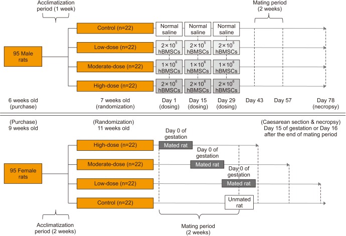
Fig. 1
Experimental design. For male rats, a 50 µL suspension of human bone marrow-derived mesenchymal stem cells (hBMSCs) (for the hBMSC injection groups) or normal saline (for the control group) was injected into the penis, 3 times at 2-week-intervals. Male and female rats of the same group were cohabitated (1:1) for 2 weeks of the mating period, which began 2 weeks after the final injection in the male rats. Mating was evaluated based on the presence of a mating plug or via a vaginal smear test twice a day during the mating period. If mating was confirmed, the day was designated as day 0 of presumed gestation. Pregnancy was confirmed based on the presence of implantation in the uterus at the time of Caesarean section. All mated and unmated female rats underwent Caesarean section on day 15 of gestation or 16 days after the end of mating period, respectively.
![]()
4. Observations of clinical signs
5. Body weight
6. Food consumption
7. Mating
8. Implantation rate and embryo mortality
9. Necropsy
10. Organ weights
11. Histopathological analysis
12. Sperm examinations
RESULTS
1. Clinical signs
2. Body weight
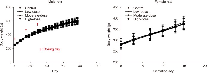
Fig. 2
Body weights of male and female rats. The body weight was analyzed using the Bartlett's test for homogeneity of variance. If equal variance was assumed, one-way analysis of variance was used, if significant, followed by the Dunnett's t-test for multiple comparisons. If equal variance was not assumed, the Kruskal–Wallis test was used, if significant, followed by the Steel's test for multiple comparisons.
![]()
3. Food consumption
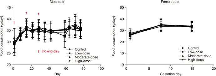
Fig. 3
Food consumption of male and female rats. The food consumption was analyzed using the Bartlett's test for homogeneity of variance. If equal variance was assumed, one-way analysis of variance was used, if significant, followed by the Dunnett's t-test for multiple comparisons. If equal variance was not assumed, the Kruskal–Wallis test was used, if significant, followed by the Steel's test for multiple comparisons.
![]()
4. Mating
Table 1
Summary of mating performance
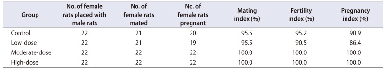
Mating index (%)=(No. of male or female rats mated/No. of female rats placed with male rats)×100
Fertility index (%)=(No. of male or female rats fertilization/No. of mated male or female rats)×100
Pregnancy index (%)=(No. of male or female rats pregnant/No. of female rats placed with male rats)×100
Mating performance was analyzed by Fisher's exact test.
![]()
5. Implantation rate and embryo mortality
Table 2
Summary of Caesarean section findings
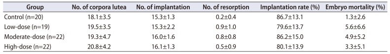
Implantation rate (%)=(No. of implantation/No. of corpora lutea)×100
Embryo mortality (%)=(No. of resorption/No. of implantation)×100
Quantitative data were expressed as mean values with standard deviations.
The number of corpora lutea, the number of implantation, and implantation rate were analyzed using the Bartlett's test for homogeneity of variance. If equal variance was assumed, one-way analysis of variance was used, if significant, followed by the Dunnett's t-test for multiple comparisons. If equal variance was not assumed, the Kruskal–Wallis test was used, if significant, followed by the Steel's test for multiple comparisons. Embryo mortality was analyzed using the Kruskal–Wallis test was used, if significant, followed by the Steel's test for multiple comparisons.
![]()
6. Necropsy findings
7. Organ weights
Table 3
Summary of absolute organ weights (unit: g)
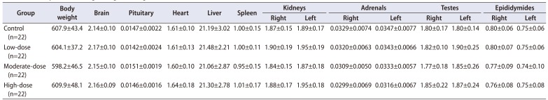
Quantitative data were expressed as mean values with standard deviations.
The organ weights were analyzed using the Bartlett's test for homogeneity of variance. If equal variance was assumed, one-way analysis of variance was used, if significant, followed by the Dunnett's t-test for multiple comparisons. If equal variance was not assumed, the Kruskal–Wallis test was used, if significant, followed by the Steel's test for multiple comparisons.
![]()
Table 4
Summary of relative organ weights (unit: g/100 g body weight)
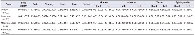
Quantitative data were expressed as mean values with standard deviations.
The organ weights were analyzed using the Bartlett's test for homogeneity of variance. If equal variance was assumed, one-way analysis of variance was used, if significant, followed by the Dunnett's t-test for multiple comparisons. If equal variance was not assumed, the Kruskal–Wallis test was used, if significant, followed by the Steel's test for multiple comparisons.
![]()
8. Histopathological analysis
9. Sperm examinations
Table 5
Summary of parameters of sperm motility in left epididymis
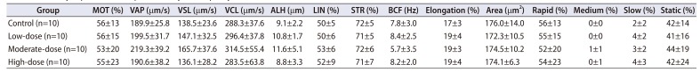
Quantitative data were expressed as mean values with standard deviations.
Parameters of sperm motility were analyzed using the Bartlett's test for homogeneity of variance. If equal variance was assumed, one-way analysis of variance was used, if significant, followed by the Dunnett's t-test for multiple comparisons. If equal variance was not assumed, the Kruskal–Wallis test was used, if significant, followed by the Steel's test for multiple comparisons.
MOT, motility; VAP, velocity of average path (VAP is computed in two passes, using an adaptive smoothing algorithm to compute running average.); VSL, velocity straight line (VSL is calculated by dividing the straight line distance between the first and last points of the track by the time interval.); VCL, velocity curvilinear (VCL is the velocity measured along the actual track of the sperm.); ALH, amplitude of lateral head displacement (ALH is the lateral head displacement amplitude, representing a measure of the width of the head swing along the sperm track.); LIN, linearity (LIN=VSL/VCL×100); STR, straightness (STR=VSL/VAP×100); BCF, beat-cross frequency (BCF is the least satisfactory parameter used to describe sperm motion.).
![]()
Table 6
Summary of sperm morphology in left epididymis
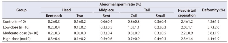
Quantitative data were expressed as mean values with standard deviations.
Sperm malformations were analyzed using the Bartlett's test for homogeneity of variance. If equal variance was assumed, one-way analysis of variance was used, if significant, followed by the Dunnett's t-test for multiple comparisons. If equal variance was not assumed, the Kruskal–Wallis test was used, if significant, followed by the Steel's test for multiple comparisons. Sperm deformity was analyzed using the Kruskal–Wallis test was used, if significant, followed by the Steel's test for multiple comparisons.
![]()
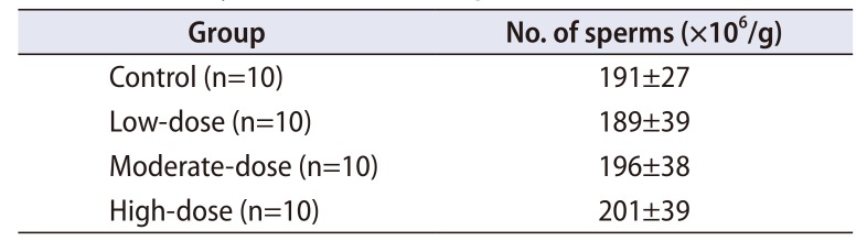
Table 7
Summary of sperm count in right testis
| Group | No. of sperms (×106/g) |
|---|---|
| Control (n=10) | 191±27 |
| Low-dose (n=10) | 189±39 |
| Moderate-dose (n=10) | 196±38 |
| High-dose (n=10) | 201±39 |
Quantitative data were expressed as mean values with standard deviations.
Sperm count was analyzed using the Bartlett's test for homogeneity of variance. If equal variance was assumed, one-way analysis of variance was used, if significant, followed by the Dunnett's t-test for multiple comparisons. If equal variance was not assumed, the Kruskal–Wallis test was used, if significant, followed by the Steel's test for multiple comparisons.
![]()

 XML Download