Understanding the pharmacokinetics of reversible metabolism

Seungil Cho; Young-Ran Yoon

doi:10.12793/tcp.2019.27.2.52

Abstract

This tutorial introduces the mathematical skills required to obtain exact and approximate solutions for reversible reactions and provides graphical insights to help understand the pharmacokinetics of reversible metabolism. The matrix method provides an easy way to derive the exact solution for the amount of each species as a function of time. The plots of the exact solutions reveal some characteristic features of the pharmacokinetic profiles of the reversible metabolism. We also describe two approximation approaches, steady-state approximation, and equilibrium approximation, to simplify the solutions. The skills and knowledge acquired through this tutorial will provide a basis for understanding more complex reversible reaction systems.

Go to :

Introduction

Reversible reactions are commonly encountered in pharmacology, chemistry, biology, chemical engineering, etc.[1 2 3 4 5 6] The influence of reversible metabolism on the pharmacokinetics of a drug and its metabolites has been the subject of considerable recent research.[5 6 7 8 9 10 11] An interesting example is the administration of chiral drugs. Two enantiomers of a chiral drug, such as ibuprofen[10] and propranolol,[11] often have different potencies and pharmacokinetic profiles.[8 9 10 11] However, one enantiomer is usually interconverted into the other within the human body.[7 8 9 10 11] When a chiral drug is administered as a racemic mixture, its bioavailability and efficacy can be incorrectly estimated if reversible reactions between two enantiomers are not taken into account.[5 6] For the determination of an appropriate dosage regimen of a drug, it is therefore important to understand the characteristics of the reversible reaction between a drug and its metabolite.

In this tutorial, we focus on the basics of the pharmacokinetics of reversible metabolism. For a simple reversible reaction scheme, we use the matrix method to get exact solutions and plot them to find characteristic relationships between the pharmacokinetic profiles of a parent drug and its metabolites. In addition, we describe two approximation approaches to deal with complex problems and examine the conditions required for the successful application of each approach.

Go to :

Theoretical analysis

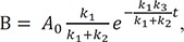
Exact solution for the kinetics of reversible reaction

Let us consider the following simple reversible reaction scheme

$A \begin{matrix} k_{1} \\ ⇄ \\ k_{2} \end{matrix} B \begin{matrix} k_{3} \\ \to \end{matrix} C,$

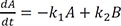
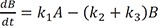
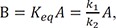
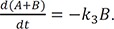
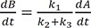
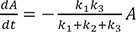
Where the first step is reversible with a forward rate constant k₁ and reverse rate constant k₂, and the second step is irreversible with the rate constant k₃. The rate constant has the units of the amount per unit time, which are omitted for simplicity in this tutorial. The rate equations are:

(1)

$\frac{d A}{d t} = - k_{1} A + k_{2} B$

(2)

$\frac{d B}{d t} = k_{1} A - (k_{2} + k_{3}) B$

(3)

$\frac{d C}{d t} = k_{3} B$

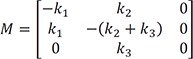
Linear ordinary differential equations can be solved using Laplace transformation or the matrix method.[2 3 7 12] We used the latter to obtain an exact solution because of its simplicity. The above expressions can be written in matrix form:

(4)

$M = [\begin{matrix} - k_{1} & k_{2} & 0 \\ k_{1} & - (k_{2} + k_{3}) & 0 \\ 0 & k_{3} & 0 \end{matrix}]$

By setting

$|\begin{matrix} - k_{1} - λ & k_{2} & 0 \\ k_{1} & - (k_{2} + k_{3}) - λ & 0 \\ 0 & k_{3} & - λ \e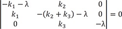nd{matrix}| = 0$

, where λ is the eigenvalue, and solving for λ, we get the following characteristic polynomial:

(5)

$λ (λ^{2} + p λ + q) = 0$

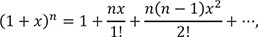
Where p = k₁ + k₂ + k₃ and q = k₁k₃. The solutions of the quadratic equation in Eq. (5) are given by

$α = \frac{p + \sqrt{p^{2} - 4 q}}{2},$

and

$β = \frac{p - \sqrt{p^{2} - 4 q}}{2} .$

The resulting eigenvalues are 0, −α, and −β. These eigenvalues are substituted into the eigenvalue equation to yield the corresponding eigenvectors of

$[\begin{matrix} 0 \\ 0 \\ 1 \end{matrix}], [\begin{matrix} β - k_{1} \\ k_{1} \\ β \end{matrix}], a n d [\begin{matrix} α - k_{1} \\ k_{1} \\ α \end{matrix}]$

, spectively.

Because the matrix M has three distinct real eigenvalues and their corresponding eigenvectors, we can express the solution as

(6)

$[\begin{matrix} A \\ B \\ C \end{matrix}] = C_{0} [\begin{matrix} 0 \\ 0 \\ 1 \end{matrix}] + C_{1} [\begin{matrix} β - k_{1} \\ k_{1} \\ β \end{matrix}] e^{- α t} + C_{2} [\begin{matrix} α - k_{1} \\ k_{1} \\ α \end{matrix}] e^{- β t}$

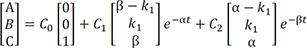
At t = 0, A = A₀ and B = C = 0, and A + B + C = A₀ at all times. Using these boundary conditions, we can solve Eq. (6) to get C₀ = A₀, C₁ = −C2 and C₁ = A₀/(β – α). Then, the final expressions for the above differential equations (1–3) are

(7)

$A = \frac{A_{0}}{β - α} \{(β - k_{1}) e^{- α t} - (α - k_{1}) e^{- β t}\}$

(8)

$B = \frac{k_{1} A_{0}}{β - α} (e^{- α t} - e^{- β t})$

(9)

$C = \frac{A_{0}}{β - α} (β - α + {α e}^{- β t} {- β e}^{- α t})$

We can compare these results to those for a consecutive two-step reaction, as described in the previous tutorial.[13] We can easily show that the latter has the eigenvalues of 0, −k₁, and −k₃, by setting k₂ = 0 in Eq. (5). The solutions for B and C, equations 8 and 9 in this study, are very similar to those for the consecutive reaction (Equations 7 and 9 in Reference,[13] respectively). Thus, the expressions for the maximum amount of B (B_max) and the time to reach the peak (t_max) can be obtained in a similar way:

(10)

$t_{m a x} = \frac{1}{β - α} \ln \frac{β}{α}$

and

(11)

$B_{m a x} = A_{0} \frac{k_{1}}{β} {(\frac{α}{β})}^{\frac{α}{β - α}} = A_{0} \frac{k_{1}}{α} {(\frac{α}{β})}^{\frac{β}{β - α}},$

respectively.

Graphical insights into the kinetics of reversible reactions

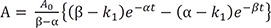
Figure 1 shows representative amount versus time curves of A, B, and C, plotted on a linear and semi-logarithmic scale for three different cases: (a) k₁ = 10, k₂ = 0.1, and k₃ = 1; (b) k₁ = 5, k₂ = 4, and k₃ = 2; (c) k₁ = 1, k₂ = 5, and k₃ = 0.2. When k₁ and k₃ are relatively larger than k₂, that is, the reverse reaction is negligible, linear plots of the amount versus time curves of A and B for the reversible reaction (Fig. 1a) look very similar to those for a consecutive irreversible reaction (see Figure 2 in Reference[13]). The semi-logarithmic plots for the former case (Fig. 1b), however, look different from those for the latter case (see Figure 3a in Reference[13]). In the former case, two curves are always parallel to each other in the elimination phase, whereas they are not in the latter case. The difference can be explained as follows. For an irreversible reaction, the amount of A is described by one exponential term, whereas for the reversible reaction, it is described by two exponential terms. For the latter, the first term in Eq. (7) or (8) decreases faster than the second term over time, because α is always larger than β. This means that the elimination phase is governed by the second term. Therefore, the first term can be neglected when t is sufficiently large. In semi-logarithmic plots of A and B, thus, both slopes for the elimination phase are linear and identical and given by –β/2.303. The y-intercepts for A and B are

$\frac{α - k_{1}}{α - β} A_{0}$

and

$\frac{k_{1}}{α - β} A_{0}$

, respectively. When 2k₁ = 2k₂ + k₃, the intercepts are the same, as shown in Figure 2. If 2k₁ < 2k₂ + k₃, the curves A and B will not cross each other. As a third case, we set k₁ = 1, k₂ = 5, and k₃ = 0.2, which satisfies this condition. It is noteworthy that the semi-logarithmic plots for this case (Fig. 3b) strongly resemble those for the consecutive irreversible reaction (see Figure 3b in Reference[13]). In the latter case, the semi-logarithmic plots of plasma concentrations versus time of A and B become parallel straight lines at large t only when the formation rate of B is much slower than its elimination rate; that is, the metabolism is formation rate-limited (FRL).[13 14 15] In addition, the intercept for [B] becomes greater than that for [A] when the distribution volume of B, V_B, is much smaller than that of A, V_A (see Figure 3c in Reference[13]). However, we need to be cautious when we apply this feature to the interpretation of the time profiles of the semi-logarithmic plots of a drug and its metabolite because this feature is commonly observed in reversible metabolic reactions. The pharmacokinetic parameters for each case, including t_max and B_max, are summarized in Table 1.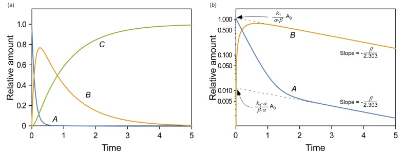

Figure 1

(a) Linear and (b) semi-logarithmic plots of the amount-time curves of A, B, or C in the reversible reaction, $A \begin{matrix} k_{1} \\ ⇄ \\ k_{2} \end{matrix} B \begin{matrix} k_{3} \\ \to \end{matrix} C$
, where k₁ = 10, k₂ = 0.1, and k₃ = 1. The abscissa and ordinate denote the time and the amount of each species, respectively, in arbitrary unit. See text for details.

undefined

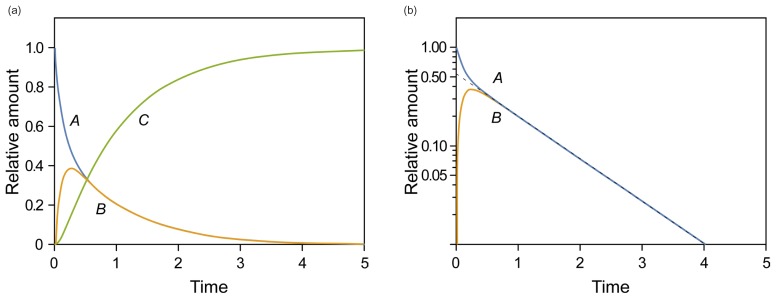Figure 2

(a) Linear and (b) semi-logarithmic plots of the amount-time curves of A, B, or C in the reversible reaction, $A \begin{matrix} k_{1} \\ ⇄ \\ k_{2} \end{matrix} B \begin{matrix} k_{3} \\ \to \end{matrix} C$
, where k₁ = 5, k₂ = 4, and k₃ = 2. The abscissa and ordinate denote time and the amount of each species, respectively, in arbitrary unit. See text for details.

undefined

Figure 3

(a) Linear and (b) semi-logarithmic plots of the amount-time curves of A, B, or C in the reversible reaction, $A \begin{matrix} k_{1} \\ ⇄ \\ k_{2} \end{matrix} B \begin{matrix} k_{3} \\ \to \end{matrix} C$
, where k₁ = 1, k₂ = 5, and k₃ = 0.2. The abscissa and ordinate denote time and the amount of each species, respectively, in arbitrary unit. See text for details.

undefined

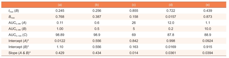
Table 1

Pharmacokinetic parameters for the following cases: (a) k₁ = 10, k₂ = 0.1, and k₃ = 1 (as in Fig. 1); (b) k₁ = 5, k₂ = 4, and k₃ = 2 (as in Figure 2); (c) k₁ = 1, k₂ = 5, and k₃ = 0.2 (as in Figure 3); (d) k₁ = 0.1, k₂ = 1, and k₃ = 5, (as in Figure 4a); (e) k₁ = 10, k₂ = 1, and k₃ = 0.1 (as in Figure 4b)

	(a)	(b)	(c)	(d)	(e)
t_max (B)	0.245	0.256	0.855	0.722	0.439
B_max	0.768	0.387	0.158	0.0157	0.873
AUC_0–∞ (A)	0.11	0.6	26	12.0	1.1
AUC_0–∞ (B)	1.00	0.5	5	0.2	10.0
AUC_0–100 (C)	98.89	98.9	69	87.8	88.9
Intercept (A)^*	0.0122	0.556	0.842	0.998	0.0924
Intercept (B)^*	1.10	0.556	0.163	0.0169	0.915
Slope (A & B)^*	0.429	0.434	0.014	0.0361	0.0394

AUC_0–∞ and AUC_0–100 represent the areas under the curve from t = 0 to t = ∞ and 100, respectively. All the intercepts and slopes (^*) were obtained from semi-logarithmic plots.

The area under the curve (AUC) is an important pharmacokinetic parameter, representing total drug exposure over time. The AUC for A and B can be obtained by directly integrating Eqs. (7) and (8) from zero to infinity, respectively, and expressed as

(12)

${A U C}_{A} = \frac{(k_{2} + k_{3}) A_{0}}{q}$

and

(13)

${A U C}_{B} = \frac{k_{1} A_{0}}{q} .$

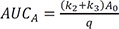
Thus, the ratio of AUC_A to AUC_B can be simplified to

$\frac{k_{2} + k_{3}}{k_{1}}$

. The AUC for C can also be calculated by integrating Eq. (9) from zero to t and given by

(14)

${A U C}_{C} = A_{0} (t - \frac{p}{q}) .$

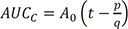
Using a time integration method,[14 16] we can obtain the relationship between AUC and rate constant or clearance, which has the units of volume (V) per unit time (CL = k × V). By separating the variables in Eqs. (7–9) and integrating both sides with respect to their respective variables, we can write the equations as follows:

(15)

$V_{A} \int_{{[A]}_{0}}^{\infty} d [A] = {- k_{1} V}_{A} \int_{0}^{\infty} [A] d t + k_{2} V_{B} \int_{0}^{\infty} [B] d t,$

(16)

$V_{B} \int_{{[B]}_{0}}^{\infty} d [B] = {k_{1} V}_{A} \int_{0}^{\infty} [A] d t - (k_{2} + k_{3}) V_{B} \int_{0}^{\infty} [B] d t,$

(17)

$V_{C} \int_{{[C]}_{0}}^{\infty} d [C] = k_{3} V_{B} \int_{0}^{\infty} [B] d t .$

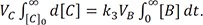
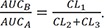
They should satisfy the following boundary conditions: [B] = [C] = 0 at t = 0; [A] = [B] = 0 and V_C × [C] = A₀ at t = ∞. By substituting k₁ = CL₁/V_A, k₂ = CL₂/V_B, and k₃ = CL₃/V_C, we get

(18)

A₀=CL₁AUC_A−CL₂AUC_B,

(19)

CL₁AUC_A=(CL₂+CL₃)AUC_B

(20)

A₀=CL₃AUC_B

Eq. (19) can be rearranged as

(21)

$\frac{{A U C}_{B}}{{A U C}_{A}} = \frac{{C L}_{1}}{{C L}_{2} + {C L}_{3}} .$

These relationships are helpful in understanding pharmacokinetic features and metabolic pathways.[14 17 18]

Approximation of the kinetics of reversible reactions

To get a good approximate solution for a reversible reaction scheme, approximation approaches have been developed and are widely used.[12 19 20] Depending upon the reactivity of the intermediate species, we can use either of two approximation approaches. One is a steady-state approximation, in which the intermediate species B is very reactive and hence short lived. This approximation is useful for explaining reactions involving radical species. The other is an equilibrium approximation, in which B is quite stable and long-lived because the equilibrium reaction proceeds faster than the product formation reaction; that is, k₁, k₂ >> k₃. For both approaches, the following condition should be satisfied:

(22)

$\frac{d B}{d t} \approx 0$

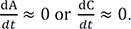
In the steady-state approximation, B is extremely unstable and very short-lived and thus is present in most of the time in extremely small amounts. By assuming that B ≈ 0, we can get a new boundary condition: A + C = A₀. From Eq. (22), Eq. (2) can be rearranged to yield:

(23)

$\frac{B}{A} = \frac{k_{1}}{k_{2} + k_{3}} ≪ 1$

For the steady-state approximation, this ratio should be very small because the amount of B is much smaller than that of A. Substituting Eq. (23) into Eq. (1) and re-arranging it for A, we have

(24)

$\frac{d A}{d t} = - \frac{k_{1} k_{3}}{k_{2} + k_{3}} A$

By separating the variables and integrating the resulting equation, we get

(25)

$A = A_{0} e^{- \frac{k_{1} k_{3}}{k_{2} + k_{3}} t}$

Using the above expression and the new boundary condition, A + C = A₀, we obtain

(26)

$C = A_{0} (1 - e^{- \frac{k_{1} k_{3}}{k_{2} + k_{3}} t})$

Now we can solve Eq. (2) for B using Eq. (26), to get

(27)

$B = A_{0} \frac{k_{1}}{k_{2} + k_{3}} e^{- \frac{k_{1} k_{3}}{k_{2} + k_{3}} t}$

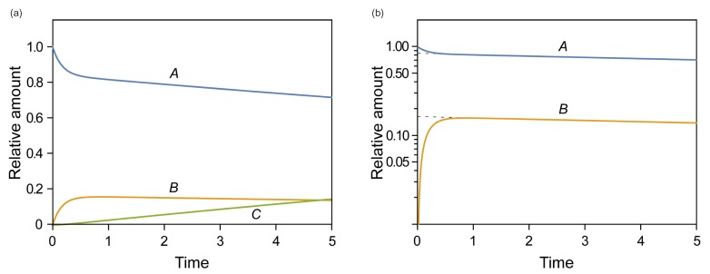
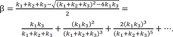
We plot the exact and approximate solutions for the case where k₁ = 0.1, k₂ = 1, and k₃ = 5 (Fig. 4a). Because

$\frac{k_{1}}{k_{2} + k_{3}} = \frac{0.1}{1 + 5} ~ 0.017 ≪ 1$

, the requirement for the steady-state approximation is satisfied. As the reaction begins, the amount of B quickly increases but is still extremely small (B_max = 0.016 at t_max = 0.72) for most of the time, as expected. As shown in Figure 4a, the approximate solutions (dashed lines) agree well with the exact solutions (solid lines).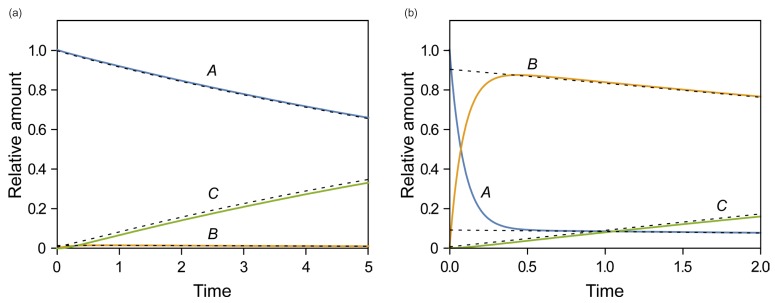

Figure 4

Linear plots of the amount-time curves of A, B, or C for the cases of (a) k₁ = 0.1, k₂ = 1, and k₃ = 5, corresponding to the steady-state approximation, and (b) k₁ = 10, k₂ = 1, and k₃ = 0.1, corresponding to the equilibrium approximation. The solid and dashed lines represent the exact and approximate solutions, respectively. The abscissa and ordinate denote time and the amount of each species, respectively, in arbitrary unit. See text for details.

For the equilibrium approximation, the reaction needs to be in pseudo-equilibrium. In such a case, we can express

(28)

$B = K_{e q} A = \frac{k_{1}}{k_{2}} A,$

Where K_eq is an equilibrium constant. Because

(29)

$\frac{d A}{d t} + \frac{d B}{d t} + \frac{d C}{d t} = 0,$

we also have

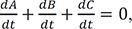
$\frac{d A}{d t} \approx 0 o r \frac{d C}{d t} \approx 0 .$

Because of the above condition, it is not feasible to directly solve Eqs. (1) and (2). Instead, we need to combine the two equations to get

(30)

$\frac{d (A + B)}{d t} = - k_{3} B .$

If we define X = A + B = A₀ – C, from Eq. (28), we can express A and B as

(31)

$A = \frac{k_{2}}{k_{1} + k_{2}} X a n d B = \frac{k_{1}}{k_{1} + k_{2}} X .$

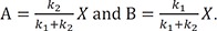
Now Eq. (30) can be solved for X to get

(32)

$X = A_{0} e^{- \frac{k_{1} k_{3}}{k_{1} + k_{2}} t}$

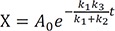
Then, we have

(33)

$A = A_{0} \frac{k_{2}}{k_{1} + k_{2}} e^{- \frac{k_{1} k_{3}}{k_{1} + k_{2}} t},$

(34)

$B = A_{0} \frac{k_{1}}{k_{1} + k_{2}} e^{- \frac{k_{1} k_{3}}{k_{1} + k_{2}} t},$

(35)

$C = A_{0} (1 - e^{- \frac{k_{1} k_{3}}{k_{1} + k_{2}} t}) .$

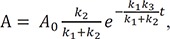
In Figure 4b, we show the plots of the exact and approximate solutions for the case where k₁ = 10, k₂ = 1, and k₃ = 0.1. Unlike in Figure 4a, the amount of B is not negligible (B_max = 0.87 at t_max = 0.44). The reaction rapidly reaches quasi-equilibrium, after which the amount of B slowly decreases. As shown in Figure 4b, the approximate solutions (dashed lines) agree well with the exact solutions (solid lines).

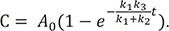
The difference between steady-state and equilibrium approximate approaches lies in the range of their applicability. [20] When we introduce an additional constraint, k₂ >> k₁ into the equilibrium approach and k₂ >> k₃ into the steady state approach, both methods will yield the same solution.[20] This relationship can be further explained by considering an approximate expression for β. Using the following binomial theorem

${(1 + x)}^{n} = 1 + \frac{n x}{1!} + \frac{n (n - 1) x^{2}}{2!} + \dots,$

we can obtain the binomial expansion of β, which yields

(36)

$β = \frac{k_{1} + k_{2} + k_{3} - \sqrt{{(k_{1} + k_{2} + k_{3})}^{2} - 4 k_{1} k_{3}}}{2} = \frac{k_{1} k_{3}}{k_{1} + k_{2} + k_{3}} + \frac{{(k_{1} k_{3})}^{2}}{{(k_{1} + k_{2} + k_{3})}^{3}} + \frac{2 {(k_{1} k_{3})}^{3}}{{(k_{1} + k_{2} + k_{3})}^{5}} + \dots .$

If k₁ + k₂ >> k₃ or k₂ + k₃ >> k₁, the second and higher order terms in the expansion can be negligible, and the first term can be further simplified to be the same as the exponent in the equilibrium approximation [see Eqs. (33–35)] or in the steady-state approximation [see Eqs. (25–27)], respectively. For a refined approximation, we can differentiate Eq. (23) for A and B with respect to time t to get

(37)

$\frac{d B}{d t} = \frac{k_{1}}{k_{2} + k_{3}} \frac{d A}{d t}$

By substituting Eqs. (3), (23), and (37) into Eq. (29) and rearranging the resulting equation, we get

(38)

$\frac{d A}{d t} = - \frac{k_{1} k_{3}}{k_{1} + k_{2} + k_{3}} A$

We expect a better approximate solution from the above equation compared with that produced by Eq. (24).

Application of the Reversible Reaction Scheme

The reversible reaction scheme is also used to describe drug distribution after rapid intravenous injection. Drug distribution within the body is often described by a two-compartment model with central and peripheral compartments.[21] In this model, an injected drug will be either eliminated or distributed within the central compartment, representing intravascular space, and the peripheral compartment, representing non-metabolizing body tissues. The distribution phase can be expressed by two linear differential equations similar to Eqs. 1 and 2.[21] The solution for drug concentration in each compartment can be obtained using a similar approach and described by two exponential terms.

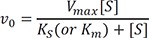
To explain the kinetics of an enzyme-catalyzed reaction, a Michaelis-Menten model has been widely used.[22 23 24] When an enzyme and a substrate form a complex, the binding of the substrate to the active site of the enzyme is non-covalent and reversible. If the conversion of the enzyme-substrate complex to a product is the rate-limiting process, the concentration of the complex can be considered to be constant. Then, the equilibrium approximation will give a hyperbolic relationship between the initial reaction rate, v_0, and substrate concentration [S], known as the Michaelis-Menten equation,

$v_{0} = \frac{V_{m a x} [S]}{K_{S} ({o r K}_{m}) + [S]}$

Where V_max is the maximum reaction rate achieved when all of the active sites are occupied by substrates. The Michaelis constant, in the original article,[22 23] is given by

$K_{S} = \frac{k_{2}}{k_{1}}$

. When a steady-state approximation is used, the constant is given by

$K_{m} = \frac{k_{2} + k_{3}}{k_{1}}$

. [24]

Go to :

Concluding remarks

We have described the mathematical approaches needed to determine the reaction kinetics of a reversible reaction system and provided graphical insights into the results. The knowledge acquired through this tutorial may help deepen the understanding of the pharmacokinetics of reversible metabolism and ultimately help with the prediction of the appropriate dose of a drug that is subject to equilibrium in a human body.

Go to :