Assessing the Optimal Cutpoint for Tumor Size in Patients with Lung Cancer Based on Linear Rank Statistics in a Competing Risks Framework

Jinheum Kim; Hon Keung Tony Ng; Seong W. Kim

doi:10.3349/ymj.2019.60.6.517

Abstract

Purpose

In clinical studies, patients may experience several types of events during follow up under the competing risks (CR) framework. Patients are often classified into low- and high-risk groups based on prognostic factors. We propose a method to determine an optimal cutpoint value for prognostic factors on censored outcomes in the presence of CR.

Materials and Methods

We applied our method to data collected in a study of lung cancer patients. From September 1, 1991 to December 31, 2005, 758 lung cancer patients received tumor removal surgery at Samsung Medical Center in Korea. The proposed statistic converges in distribution to that of the supremum of a standardized Brownian bridge. To overcome the conservativeness of the test based on an approximation of the asymptotic distribution, we also propose a permutation test based on permuted samples.

Results

Most cases considered in our simulation studies showed that the permutation-based test satisfied a significance level of 0.05, while the approximation-based test was very conservative: the powers of the former were larger than those of the latter. The optimal cutpoint value for tumor size (unit: cm) prior to surgery for classifying patients into two groups (low and high risks for relapse) was found to be 1.8, with decent significance reflected as p values less than 0.001.

Conclusion

The cutpoint estimator based on the maximally selected linear rank statistic was reasonable in terms of bias and standard deviation in the CR framework. The permutation-based test well satisfied type I error probability and provided higher power than the approximation-based test.

Go to :

INTRODUCTION

In clinical studies, patients are often classified into low- and high-risk groups based on prognostic factors. For example, serum creatinine level might be an important prognostic factor for rejection after renal transplantation. If a patient has no acute rejection and a low serum creatinine level for six months after transplantation, administered steroids are often withdrawn. A cutpoint value of 2.0 (unit: mg/dL) is commonly used as a threshold for serum creatinine to make this clinical decision. In this case, patients with a serum creatinine level less than or equal to 2.0 could be classified into the low-risk group and those with level greater than 2.0 into the high-risk group.

When an event of interest is survival time, one of the most popular procedures is to minimize the p value associated with the log-rank statistic. A considerable amount of work has dealt with censored outcomes based on a maximally selected linear rank statistic.1 2 3 4 5 These methods can be applied to situations with only one type of event; however, patients may experience several types of events during follow up, which may compel an analysis with the competing risks (CR) framework. Woo, et al.6 proposed a method to determine a cutpoint value of a prognostic factor on censored outcomes in the presence of CR. They also proposed a maximally selected Gray's test statistic7 8 for testing whether there is an association between the event of interest and the prognostic factor, and approximated the asymptotic distribution using the arguments.4 9 However, it turned out that the test procedure was conservative under moderate to heavy censoring.6 In this article, we propose test statistics to circumvent these shortcomings.

This article is organized in the following manner. We first propose a cutpoint estimator for a prognostic factor that produces the largest difference in the event of interest between individuals in low- and high-risk groups under a CR framework. Two different procedures are proposed to test whether an association between the event of interest and the prognostic factor is statistically significant at the estimated cutpoint of the prognostic factor. Simulations are conducted to investigate the performance of the cutpoint estimator in terms of bias and precision and the efficiency of the proposed tests in terms of power. We also analyze lung cancer data collected from Samsung Seoul Hospital in Korea to illustrate our proposed methodologies. Finally, brief discussions are provided.

Go to :

MATERIALS AND METHODS

Materials

From September 1, 1991 to December 31, 2005, 758 lung cancer patients underwent tumor removal surgery at Samsung Medical Center in Korea. This study was conducted over more than 16 years and the observed follow-up times ranged from 0.3 to 195 months. In this study, relapse after the surgical process corresponds to the event of interest, and death corresponds to a CR. Among the patients, 580 relapsed (76.5%), 65 died without relapse (8.6%), and 113 were censored (14.9%). The prognostic factor was tumor size (unit: cm) at surgery, which ranged from 0 to 19. A box plot of tumor size with the five numbers is displayed in Fig. 1. Moreover, summary statistics of time to event occurrence and tumor size are presented in Table 1 depending on the event type, such as censoring, relapse, or death.

Fig. 1

Box plot of tumor size with the five numbers.

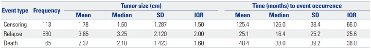
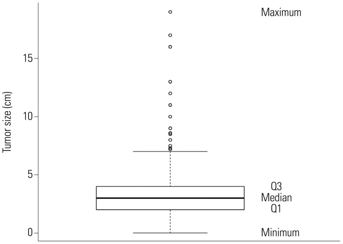
Table 1

Summary Statistics of Time to Event Occurrence and Tumor Size Depending on the Event Type

Event type	Frequency	Tumor size (cm)				Time (months) to event occurrence
Event type	Frequency	Mean	Median	SD	IQR	Mean	Median	SD	IQR
Censoring	113	1.78	1.60	1.287	1.50	125.4	126.0	38.4	66.0
Relapse	580	3.65	3.25	2.120	2.00	25.1	16.4	25.2	25.6
Death	65	2.37	2.10	1.423	1.60	48.4	38.0	39.2	36.0

SD, standard deviation; IQR, interquartile range.

Models and notations

Let X, Y, and C be the time of the event of interest, the time of CR, and a censoring time, respectively. Let δ=1 if the event of interest occurred, 2 if the CR occurred, and 0 if censored. Let

{D_i=(T_i=X_i⋀Y_i⋀C_i,δ_i,Z_i):i=1,2,…,n}

be observed data, where Z_i is a continuous prognostic factor. Suppose that

0=t₍₀₎<t₍₁₎<t₍₂₎<···<t_(m)<t_(m+1)=∞(m≤n)

are the ordered distinct times at which the event of interest occurs and that

D(t_(u))={u₁,u₂,…u_{d_u}}

is the set of labels of subjects that fail at t_(u), u=1, 2, …, m. In addition, suppose that

$C (t_{(u)}) = {u_{1}^{'}, u_{2}^{'}, \dots, u_{c_{u}}^{'}}$

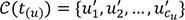
is the set of labels of subjects censored or failed due to CR in the interval [t_(u), t_(u+1)), u=0, 1, …, m.

For a fixed value of µ, set g=1 if Z≤µ and 1 otherwise. Let d_g,u(µ) and r_g,u(µ) denote the number of subjects to whom the event of interest occurs at t_(u) and the number of subjects who are at risk up to time t_(u) in group g, respectively. Let r_u=r_1,u(µ)+r_2,u(µ). Let F_g,µ(t) be the cumulative incidence function (CIF) for the event of interest and S_g,µ(t) be the survival function of being free from any event at t in group g, respectively. The estimated CIF⁸ of F_g,µ(t) is given by

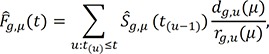
${\hat{F}}_{g, µ} (t) = \sum_{u : t_{(u)} \leq t} {\hat{S}}_{g, µ} (t_{(u - 1)}) \frac{d_{g, u (µ)}}{r_{g, u} (µ)},$

where Ŝ_g,µ(t) is the Kaplan-Meier estimator for S_g,µ(t).10 Define

$w_{g, u} (µ) = \frac{1 - {\hat{F}}_{g, µ} (t_{(u - 1)})}{{\hat{S}}_{g, µ} (t_{(u - 1)})}$

as a correction factor at t_(u) in group g. Let r̃_g,u(µ)=w_g,u(µ)r_g,u(µ) and r̃_u(µ)=r̃_1,u(µ)+r̃_2,u(µ). Define the score for a subject in D(t_(u)) at t_(u) as

$a_{l, u} (µ) = 1 - \sum_{j = 1}^{u} \{\sum_{g = 1}^{2} I_{l, g} (µ) w_{g, j} (µ)\} \frac{d_{j}}{{\tilde{r}}_{j} (µ)} for l \in D (t_{(u)}),$

where I_i,g(µ)=1 if subject i is a member of group g and 0 otherwise. Also, define the score for a subject in C(t_(u)) at t_(u) as

$A_{l^{'}, u} (µ) = \{\begin{matrix} 0, u = 0; \\ - \sum_{j = 1}^{u} \{\sum_{g = 1}^{2} I_{l^{'}, g} (µ) w_{g, j} (µ)\} \frac{d_{j}}{{\tilde{r}}_{j} (µ)}, u = 1,2, \dots, m \end{matrix}$

for l′∈C(t_(u)). We call these scores the Gray-statistic-type scores and denote ā_µ by their average score.

Maximally selected rank statistics

The testing problem of interest is the independence of X and Z, setting up the null hypothesis as

(1)

H₀:P(X≤t|Z≤µ)=P(X≤t|Z>µ)

for all t∈(0,∞) and all cutpoints µ in the prognostic factor Z. It was showed that, for a fixed value of µ, the Gray's test statistic7 8 for testing the hypothesis of (1) is equivalent to a linear rank statistic,6

$L_{µ} = \sum_{u = 1}^{m} \sum_{l \in D (t_{(u)})} I_{l, 1} (µ) a_{l, u} (µ) + \sum_{u = 0}^{m} \sum_{l' \in C (t_{(u)})} I_{l^{'}, 1} (µ) A_{l^{'}, u} (µ) .$

Let

$H_{z} (µ) = n^{- 1} \sum_{i = 1}^{n} I \{Z_{i} \leq µ\}$

denote the empirical distribution function of the prognostic factor Z. Let m_µ=nH_Z(µ) and n_µ=n−m_µ. Following the arguments,1 2 5 under H₀, given the scores, the expectation and the variance of L_µ are

$E (L_{µ}| Z) = \frac{m_{u}}{n} \sum_{u = 1}^{m} \{\sum_{l \in D (t_{(u)})} a_{l, u} (µ) + \sum_{l' \in C (t_{(u)})} A_{l^{'}, u} (µ)\} = m_{µ} {\bar{a}}_{µ}$

and

$v (L_{µ}| Z) = \frac{m_{µ} n_{µ}}{n (n - 1)} \{\sum_{u = 1}^{m} \sum_{l \in D (t_{(u)})} {(a_{l, u} (µ) - {\bar{a}}_{µ})}^{2} + \sum_{u = 0}^{m} \sum_{l' \in C (t_{(u)})} {(A_{l^{'}, u} (µ) - {\bar{a}}_{µ})}^{2}\} .$

Then, the standardized statistic of L_µ is defined as

$T_{µ} = \frac{L_{µ} - E (L_{µ}| Z)}{\sqrt{V (L_{µ}| Z)}} .$

Under H₀, T_µ is asymptotically normally distributed using the arguments.11

Let ξ(ε,Z)=min {µ:H_z(µ)≥ε}. We restrict the possible cutpoints to an interval [ξ(ε₁,Z),ξ(ε₂,Z)] with 0<ε₁<ε₂<1. In the same fashion,1 2 5 we define a cutpoint estimator µ̂(ε₁,ε₂) as the value of µ that yields the maximum of the absolute of T_µ, i.e.,

$\hat{µ} (ε_{1}, ε_{2}) = min \{{argmax}_{µ \in [ξ (ε_{1}, Z), ξ (ε_{2}, Z)]} |T_{µ}|\} .$

In addition, we define a maximally selected rank statistic as

$Q (ε_{1}, ε_{2}) = \binom{max}{µ \in [ξ (ε_{1}, Z), ξ (ε_{2}, Z)]} |T_{µ}| .$

From the arguments,1 2 5 the asymptotic distribution of Q(ε₁,ε₂) is equivalent to the distribution of the supremum of a standardized Brownian bridge. Thus, the approximation12 under H₀ gives

(2)

$P r (Q (ε_{1}, ε_{2}) \geq q) \approx \frac{4 ϕ (q)}{q} + ϕ (q) (q - \frac{1}{q}) log (\frac{ε_{2} (1 - ε_{1})}{(1 - ε_{2}) ε_{1}}), q \in (0, \infty),$

where ϕ(·) denotes a standard normal density.

However, as shown in Table 2, the testing procedure based on the approximation of (2) seems to be conservative. Instead, we propose a permutation test based on B permuted samples by permutingthe observed values of the prognostic factor Z. To be specific, denote Q_b(ε₁,ε₂) by the b^th(b=1, 2, …, B) permuted value of Q(ε₁,ε₂) based on

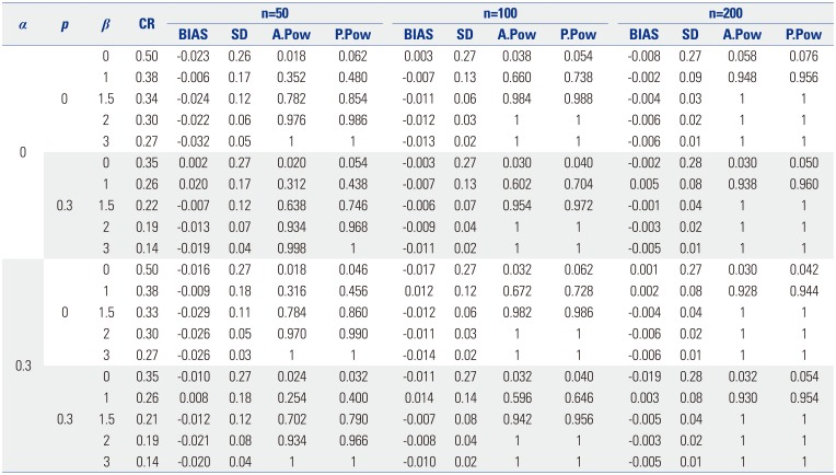
Table 2

The Proportion of CR, BIAS, and SD of the Cutpoint Estimator μ̂ and the A.Pow and P.Pow Power of the Proposed Test Statistic Q(ε₁,ε₂) for Each Combination α of p and When n=50, 100, and 200

α		β	CR	n=50				n=100				n=200
α		β	CR	BIAS	SD	A.Pow	P.Pow	BIAS	SD	A.Pow	P.Pow	BIAS	SD	A.Pow	P.Pow
0	0	0	0.50	−0.023	0.26	0.018	0.062	0.003	0.27	0.038	0.054	−0.008	0.27	0.058	0.076
		1	0.38	−0.006	0.17	0.352	0.480	−0.007	0.13	0.660	0.738	−0.002	0.09	0.948	0.956
		1.5	0.34	−0.024	0.12	0.782	0.854	−0.011	0.06	0.984	0.988	−0.004	0.03	1	1
		2	0.30	−0.022	0.06	0.976	0.986	−0.012	0.03	1	1	−0.006	0.02	1	1
		3	0.27	−0.032	0.05	1	1	−0.013	0.02	1	1	−0.006	0.01	1	1
	0.3	0	0.35	0.002	0.27	0.020	0.054	−0.003	0.27	0.030	0.040	−0.002	0.28	0.030	0.050
		1	0.26	0.020	0.17	0.312	0.438	−0.007	0.13	0.602	0.704	0.005	0.08	0.938	0.960
		1.5	0.22	−0.007	0.12	0.638	0.746	−0.006	0.07	0.954	0.972	−0.001	0.04	1	1
		2	0.19	−0.013	0.07	0.934	0.968	−0.009	0.04	1	1	−0.003	0.02	1	1
		3	0.14	−0.019	0.04	0.998	1	−0.011	0.02	1	1	−0.005	0.01	1	1
0.3	0	0	0.50	−0.016	0.27	0.018	0.046	−0.017	0.27	0.032	0.062	0.001	0.27	0.030	0.042
		1	0.38	−0.009	0.18	0.316	0.456	0.012	0.12	0.672	0.728	0.002	0.08	0.928	0.944
		1.5	0.33	−0.029	0.11	0.784	0.860	−0.012	0.06	0.982	0.986	−0.004	0.04	1	1
		2	0.30	−0.026	0.05	0.970	0.990	−0.011	0.03	1	1	−0.006	0.02	1	1
		3	0.27	−0.026	0.03	1	1	−0.014	0.02	1	1	−0.006	0.01	1	1
	0.3	0	0.35	−0.010	0.27	0.024	0.032	−0.011	0.27	0.032	0.040	−0.019	0.28	0.032	0.054
		1	0.26	0.008	0.18	0.254	0.400	0.014	0.14	0.596	0.646	0.003	0.08	0.930	0.954
		1.5	0.21	−0.012	0.12	0.702	0.790	−0.007	0.08	0.942	0.956	−0.005	0.04	1	1
		2	0.19	−0.021	0.08	0.934	0.966	−0.008	0.04	1	1	−0.003	0.02	1	1
		3	0.14	−0.020	0.04	1	1	−0.010	0.02	1	1	−0.005	0.01	1	1

CR, competing risk; BIAS, bias; SD, standard deviation; A.Pow, approximated power; P.Pow, permutation-based power.

{D_b,i=(T_i, δ_i, Z_bi):(b₁, b₂, …, b_n)∈P_n},

where P_n is a set of all permutations of integers 1 to n. Suppose that the value of Q(ε₁,ε₂) based on the observed data set {D_i:i=1, 2, …, n} is q₀. Then, the probability in the left-hand side of (2) is empirically determined by

$\frac{1}{B} \sum_{b = 1}^{B} I \{Q_{b} (ε_{1}, ε_{2}) \geq q_{0}\},$

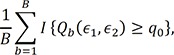
called the empirical p value corresponding to the observed value of q₀.

Go to :

RESULTS

Simulation studies

We performed simulations to investigate the finite-sample performance of the proposed methods in terms of bias and standard deviation (SD) of the cutpoint estimator and the empirical power of the maximally selected test statistics. We generated a time to the event of interest (X) and time to a CR (Y) using Gumbel's bivariate exponential distribution13 14 with degree of dependency α set as 0 and 0.3. We generated a non-informative censoring time C from an exponential distribution with a hazard rate of λ(>0), which was determined to satisfy P(C<X⋀Y)=p, where p denotes the censoring fraction. We set p=0 and 0.3. We also generated the prognostic factor Z from a uniform distribution U(0,1) and set the true cutpoint value µ as 0.5. We set ε₁=0.1 and ε₂=0.9. The effect size θ=exp(β) was the relative risk between the two groups of patients, where Z was greater than or less than or equal to µ. We set β as 0, 1, 1.5, 2, and 3: β=0 corresponded to the null hypothesis and β=1, 1.5, 2, and 3 corresponded to the alternative hypotheses. We considered four combinations of α and p: (α,p)=(0,0), (0,0.3), (0.3,0), (0.3,0.3). We performed 500 replications for each configuration of α and p with sample sizes of 50, 100, and 200. We also permuted each sample 250 times to obtain the empirical null distribution of Q(ε₁,ε₂). Fig. 2 depicts the empirical p values of the proposed test Q(ε₁,ε₂) based on a simulated sample against the number b of permutation times for each combination of α and p under H₀:β=0. As shown in Fig. 2, the number B=250 of permutation times was chosen as acceptable regardless of the sample size and the combinations of α and p. See the work6 for details of the data generation procedures. Fig. 3 depicts the empirical distribution function of μ̂ based on 2000 replications, with the sample size of 100 for each combination of α and p when β=0, 1, 1.5, 2, and 3. As expected, regardless of the combinations of α and p, the distribution of μ̂ is centered around the true cutpoint value 0.5 of µ as β increases from 0 to 3.

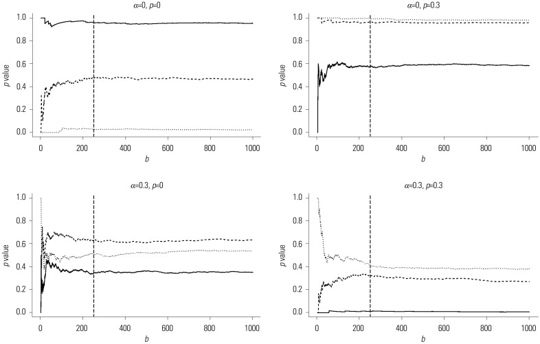Fig. 2

Empirical p values of the proposed test Q(ε₁,ε₂) calculated from a simulated sample against the number of permutation times b for four combinations of α and p under H₀:β=0 when ε₁=0.1 and ε₂=0.9: solid line for n=50, dashed line for n=100, dotted line for n=200, and the long-dashed vertical line at the 250th permutation time.

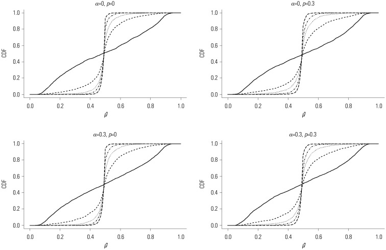Fig. 3

Empirical distribution function (CDF) of the cutpoint estimator μ̂ for the combinations of α and p when n=100: the solid line for β=0, the dashed line for β=1, the dotted line for β=1.5, the dotted and dashed line for β=2, and the long-dashed line for β=3. CDF, cumulative distribution function.

Table 2 displays the proportion of CR, the bias (Bias) and SD of the cutpoint estimator μ̂, and the approximated (A.Pow) and permutation-based (P.Pow) power of the proposed test statistic Q(ε₁,ε₂). These are based on 500 replications and 250 permutations for each combination of α and p when n=50, 100, and 200. As expected, as β increases, the SD of μ̂ decreases gradually, and both A.Pow and P.Pow converge to 1 regardless of the combination of α and p and sample size n. For a fixed value of β, as n increases, both Bias and the SD of μ̂ decrease; also, both A.Pow and P.Pow increase for any combination of α and p. The permutation-based test (P.Pow), included in the interval (0.031,0.069), satisfies a significance level of 0.05 for most cases, while the approximated test (A.Pow) is very conservative. Furthermore, P.Pow is larger than A.Pow regardless of the combination of α and p and sample size n.

Real data analysis

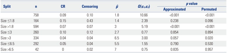
Based on the proposed test statistic Q(ε₁,ε₂), we split the patients into two groups for relapse, a high-risk group and a low-risk group, to apply different treatments to each group. We set ε₁ and ε₂ as 0.1 and 0.9, respectively. As shown in Table 3, at the first split of 758 patients, the criterion was tumor size of 1.8, and the CIFs for relapse of the two groups were different (p value<0.001). We further investigated whether the patients within each subgroup were homogeneous in experiencing relapse after surgery in terms of Q(ε₁,ε₂). The group with a tumor size less than or equal to 1.8 was statistically homogeneous (p value=0.096), while the group having tumor size greater than 1.8 was not homogeneous (p value<0.001). In the same way, we applied a binary split of only the group with a tumor size greater than 1.8. The next split criterion was a tumor size of 3, and only the group with a tumor size greater than 3 was not homogeneous (p value=0.020). The third split was 6.5, and both groups, tumor size less than or equal to 6.5 or greater than 6.5, were homogeneous with p values of 0.530 and 0.957, respectively. The top left panel of Fig. 4 depicts the standardized linear rank statistics T_µ against tumor size (solid line). The 1st, 10th, 90th, and 99th quantile points of tumor size along with the estimated cutpoint μ̂ of 1.8 are indicated on the axis of tumor size with symbols of black square, black circle, black triangle, and black diamond, respectively. In the top right panel, the CIFs of two groups, tumor size greater than 1.8 (dashed line) and less than or equal to 1.8 (solid line), are displayed. In the same way, plots in the second and third rows of Fig. 4 are respectively drawn with the subgroups of 594 patients having tumor size greater than 1.8 and of 334 patients having tumor size greater than 3. In summary, we could classify the patients with tumor size less than or equal to 1.8 into a low-risk group, while the patients included in a high-risk group (i.e., having tumor size more than 1.8) could be further classified into three subgroups, lowest, moderate, and highest high-risk groups, depending on tumor sizes at surgery of 1.8 to 3, 3 to 6.5, and over 6.5, respectively.

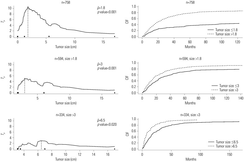Fig. 4

Plot of standardized linear rank statistic and cumulative incidence function (CIFs) of two groups classified depending on the estimated cutpoint. Left panel: standardized linear rank statistic T_µ against tumor size (solid line), estimated cutpoint (dashed line), and the 1st, 10th, 90th, and 99th quantile points of tumor size of each sub-sample (black square, black circle, black triangle, and black diamond in order). Right panel: CIF for the event time of interest of two groups, ≤ and > μ̂.

Table 3

Split Criterion of the Covariate Size, the Number of Patients of Each Node, the Estimated Cutpoint μ̂, the Proposed Test Statistic Q(ε₁,ε₂), and Approximated and Permutation-Based p values

Split	n	CR	Censoring	μ̂	Q(є₁,є₂)	p value
Split	n	CR	Censoring	μ̂	Q(є₁,є₂)	Approximated	Permuted
	758	0.09	0.10	1.8	10.66	<0.001	<0.001
Size ≤1.8	164	0.15	0.43	1.4	2.39	0.238	0.096
Size >;1.8	594	0.07	0.07	3	5.19	<0.001	<0.001
Size ≤3	260	0.10	0.12	2.7	0.77	0.854	0.894
Size >;3	334	0.04	0.04	6.5	3.00	0.057	0.020
Size ≤6.5	292	0.05	0.04	5.5	1.55	0.790	0.530
Size >;6.5	42	0	0.02	7	0.75	0.835	0.957

CR, competing risk.

Go to :

DISCUSSION

Based on a maximally selected linear rank statistic, we estimated a cutpoint for a continuous prognostic factor that produced the largest difference in the event of interest between individuals in high- and low-risk groups in a CR framework. Approximation-based and permutation-based tests were proposed to test an association between the event of interest and the prognostic factor at the estimated cutpoint of the prognostic factor. The permutation-based test procedure was proposed to overcome the conservativeness of the test based on the approximation of the asymptotic distribution of the maximally selected rank statistic. Simulation results showed that the SD of the estimated cutpoint decreased as the association between the event of interest and the prognostic factor became stronger, regardless of the combination of degree of dependency between two CR and a censoring fraction. Moreover, most cases showed that the permutation-based test satisfied a significance level of 0.05, while the approximated test was very conservative: the powers of the former were larger than those of the latter. We applied our method to data collected from a study on lung cancer patients. We used tumor size prior to surgery for classifying the patients into two groups (low and high risks for relapse). Based on the results, the optimal cutpoint value of tumor size (unit: cm) was 1.8 with ε₁=0.1 and ε₂=0.9. In addition, the times to relapse between subgroups of patients with tumor size less than or equal to 1.8 (low risk of relapse) and more than 1.8 (high risk of relapse) were significantly different (p value <0.001). The patients with tumor size over 1.8 could also be further classified into three subgroups: those with tumor size of 1.8 to 3 (lowest high risk of relapse), 3 to 6.5 (moderate high risk of relapse), and over 6.5 (highest high risk of relapse).

Following the argument,7 we also defined the risk set of the i^th subject at time t as

$Y_{i}^{G} (t) = \frac{1 - F (t)}{S (t)} I (t \leq T_{i})$

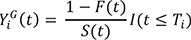
(called an adjusted method). However, since the process

$Y_{i}^{G} (t)$

excludes the contribution of the subjects who are censored by an earlier occurrence of the competing risks than an event of interest, as suggested by a referee, we could replace this process by the following process,15

(3)

$Y_{i}^{F & G} (t) = I (t \leq T_{i}) + I (X_{i} ⋀ Y_{i} \leq C_{i}) \frac{\hat{G} (t -)}{\hat{G} ((X_{i} ⋀ Y_{i}) -)} I (X_{i} ⋀ Y_{i} < t, δ_{i} = 2) .$

Here, Ĝ(t) is the Kaplan-Meier estimator of the censoring survival function G(t)=P(C>t).10 It is called Ĝ(t−)/Ĝ((X_i⋀Y_i)−) in the second term of (3) the inverse probability of censoring weighing (called an IPCW method). In the future, both the adjusted and IPCW methods will be compared with extensive simulations. Furthermore, our proposed approach can be extended to cases of CR with multiple prognostic factors. As a matter of fact, for the survival data with K(≥2) prognostic factors, Lausen, et al.5 proposed an adjusted minimal p-value approach. However, under the CR frameworks, it may not be straightforward to derive analytically the asymptotic distribution of the minimum of Q(k;ε₁,ε₂) over k(k=1, 2, …, K), where Q(k;ε₁,ε₂) denotes the value of Q(ε₁,ε₂) corresponding to the k^th prognostic factor. As an alternative, an empirical test analogous to the permutation test presented in the “maximally selected rank statistics” section would be applied to the CR data with multiple prognostic factors.

Go to :