

 PDF
PDF ePub
ePub Citation
 Print
Print


INTRODUCTION
Interest in the quantification of spatial and temporal heterogeneity within solid malignancies on medical imaging has steadily grown over the past several years (12). In particular, computed tomography (CT) texture analysis (CTTA), initially developed in an attempt to provide an objective, quantitative assessment of tumor heterogeneity by analyzing the distribution of pixel values on CT images, has increasingly garnered attention as a potential quantitative biomarker of tissue heterogeneity (345). Previous studies have demonstrated that CTTA parameters are significantly associated with histopathologic features and clinical outcomes in a variety of primary and metastatic tumors (46) and that it has utility in various non-oncologic applications, including hepatic fibrosis (478). However, the majority of CTTA studies performed thus far were retrospective in manner, using CT images collected over years (9101112); therefore, various CT scanners using various scanning techniques and reconstruction algorithms were jointly analyzed. A potential problem related to the inconsistent use of CT scanners or reconstruction algorithms is that it may introduce statistical artifacts into the images, thus failing to identify true tissue heterogeneity (131415). Therefore, to establish a clinical level of credibility for CTTA, it is crucial to investigate the impact of different reconstruction methods and scanning techniques on CT images.
Over the past several years, as the number of CT examinations has increased globally, concern over radiation exposure has risen; therefore, various new techniques have been developed to reduce the radiation dose (16). One of such dose reduction approach is the use of iterative reconstruction (IR) algorithms. Model-based, the full IR method has specifically demonstrated a higher degree of noise reduction, enabling significant radiation dose reduction, as it combines many more iterations using complex mathematics than hybrid IR methods (17). However, as model-based IR is based upon a different statistical metric, it is well known to radiologists that the resultant reconstructed images have a different morphology, presenting a mildly blurred and pixelated texture, compared to those reconstructed with either filtered back projection (FBP) or the hybrid IR (181920). Several previous studies have further suggested that such image blurring may affect their quantitative measurement on CT images (122122). Other studies have also shown that these reconstruction algorithms could affect both the extraction and analysis of quantitative imaging features of focal liver lesions, lung nodules, and renal stones (1221). Nonetheless, the impact of reconstruction methods on imaging heterogeneity and texture analysis, especially in the liver parenchyma, has not yet been elucidated.
Therefore, in the present study, we aimed to evaluate the impact of reconstruction methods on the CTTA features of the liver parenchyma by comparing FBP, hybrid IR (iDOSE4), and model-based IR (IMR) methods, as well as the intra- and inter-observer reliability of CTTA, to assess its clinical usefulness.
Go to : 
MATERIALS AND METHODS
This retrospective study was approved by the Institutional Review Board of our hospital. Because all clinical data and CT images were obtained retrospectively from medical records, the requirement for informed consent was waived.
Study Population
A search of our picture archiving and communication system database revealed that 649 patients had undergone liver CT using a single CT scanner at our hospital from Oct. 2016 to Mar. 2017. The inclusion criteria of this study were: (a) patients who had available CT images reconstructed with FBP, hybrid, and model-based IR techniques; and (b) those who had evaluable hepatic parenchyma. Those who met any of the following criteria were then excluded from the study population: (a) history of any non-surgical treatment for hepatocellular carcinoma (HCC) (n = 398), (b) history of surgical treatment of the liver within 6 months prior to the scanning date (n = 9), and (c) diffuse/infiltrative HCC or multiple (> 10) focal liver lesions (n = 15). Among the 227 remaining patients, 191 were clinically diagnosed with chronic liver disease (CLD), 24 of whom had a pathologic diagnosis of CLD, including hepatitis B-related liver cirrhosis (LC) (n = 18), cryptogenic LC (n = 2), hepatitis C-related LC (n = 1), alcoholic LC (n = 1), primary biliary cholangitis (n = 1), and severe fatty liver disease (n = 1). Of the others, 34 patients with no medical record of CLD and with a radiologic interpretation compatible with a normal liver were included and classified as the normal liver group; 76% of them had focal hepatic lesions such as hemangioma or cyst (n = 26). The other patients had a previous history of early stage cancer and had undergone follow-up CT imaging (n = 8).
Finally, 58 patients (men:women = 25:33; mean age, 56.88 ± 11.84 years) were included in our study population. There were 16 men and eight women in the CLD group (mean age, 57.33 ± 8.82 years), and nine men and 25 women in the normal liver group (mean age, 56.56 ± 13.69 years).
CT Image Acquisition
All CT examinations were performed on a 256-slice MDCT machine (Brilliance-iCT; Philips Healthcare, Cleveland, OH, USA) at our hospital. The liver CT protocol was composed of four phases: pre-contrast, arterial phase (AP), portal venous phase (PVP), and delayed phase. CT scanning was performed using the following parameters; tube voltage, 100 kVp; tube current-time products, 280 mAs; detector collimation, 128 × 0.625 mm; rotation time, 0.5 seconds; pitch, 1.0; slice thickness, 3 mm. A nonionic contrast material, iobitridol (Xenetix 350; Guerbet Korea, Seoul, Korea) was injected at a dose of 520 mg/kg of body weight using a power injector (Stellant D; Medrad, Warrendale, PA, USA) for 30 seconds at a rate of 2.1–4.3 mL/s according to body weight. Timing for the PVP scan was determined using the bolus tracking technique; that is, AP imaging was automatically performed 17 seconds after the attenuation coefficient of the abdominal aortic blood reached 100 Hounsfield units. PVP images were acquired 70 seconds after the start of contrast media administration.
CT Image Reconstruction
The obtained CT images were automatically reconstructed using three different methods including FBP, hybrid IR (iDOSE4), and model-based IR (IMR). For hybrid IR, the standard level 4 setting (50%/50% blend of IR/FBP) of iDOSE4 was applied, and for model-based IR, IMR at level 1, the low level of noise reduction setting, was used. The choice of IMR level 1 was based on a previous investigation (19).
CTTA
The single slice axial image at which portal vein bifurcation was best visualized was selected from AP and PVP images by one radiologist (with two years of clinical experience), and reconstructed using three different reconstruction methods. Thereafter, the first reviewer (with one year of clinical experience) performed CTTA using the selected images by delineating a region of interest (ROI) in the right lobe of the liver and by running commercially available software, applying the filtration-histogram statistic-based method offered by TexRAD. Specifically, a circular ROI was drawn with the diameter as long as the horizontal axis of the vertebral body shown on the sliced image with an effort to avoid large vessels or ductal structures. The ROIs were re-drawn for each reconstructed image. An example of the filtration-histogram texture analysis process performed by TexRAD is depicted in Figure 1.
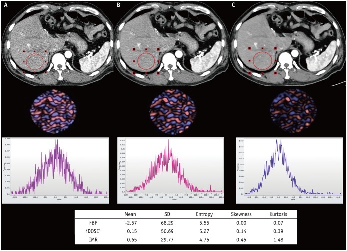 | Fig. 1Examples of filtration-histogram texture analysis process by TexRAD.First row CT images represent different reconstruction algorithms, (A) FBP, (B) iDOSE4, and (C) IMR, respectively. Second row displays processed images with fine filter value of 2. Third row displays histograms showing pixel distribution of filtered images. Table includes estimated texture feature parameters from each reconstruction algorithm. CT = computed tomography, FBP = filtered back projection, SD = standard deviation
|
To assess inter- and intra-observer reliability, the CTTA procedure was repeated using the selected images reconstructed with the FBP method. For the inter-observer reliability test, another attending radiologist (with four years of clinical experience) performed CTTA independently in a blinded manner. For the intra-observer reliability test, the first reviewer repeated the CTTA procedure 1 month after the initial analysis.
For CTTA, spatial filters, which evaluate the ROI at a different scale with object radii of different size, denoted by spatial scaling factors (SSF) of 0 to 6, were applied. SSF 0 indicates no filtration, SSF 2, 4, and 6 indicate a 2-mm, 4-mm, and 6-mm radius which represent fine, medium, and coarse filters, respectively. All filtered images were obtained using the Laplacian of the Gaussian spatial band-pass filter. Histograms of the pixel values were quantified using standard descriptors such as the mean attenuation, standard deviation (SD), entropy, skewness, and kurtosis. The mean indicates the average of pixels within the ROI. SD was the measure of how much variation or dispersion exists from the mean value (6). Entropy is a parameter that reflects the irregularity or complexity of the pixel intensities (45), skewness is a measure of the asymmetry of the histogram, reflecting the average brightness of highlighted objects, and kurtosis is a measure of the peakedness of the histogram (6).
Statistical Analysis
For comparisons between the three reconstruction methods, repeated-measures analysis of variance with Bonferroni's correction was used, and the independent t test was performed to evaluate the difference between the normal liver group and CLD group. To assess the inter-observer and intra-observer reliability of CTTA, the intraclass correlation coefficient (ICC), defined as the proportion of the total error not associated with measurement error, was calculated. ICCs of < 0.40, 0.40–0.75, and 0.76–1.00 signified poor, moderate, and excellent agreement, respectively (23). For all studies, a p value < 0.05 was considered to indicate a statistically significant difference. All statistical analyses were performed using commercially available software (MedCalc version 17.4; MedCalc Software, Ostend, Belgium; and IBM SPSS, version 21; IBM Corp., Armonk, NY, USA).
Go to :
RESULTS
Comparison According to Reconstruction Methods
The CT texture parameters of the liver parenchyma according to reconstruction methods and filter values are summarized in Tables 1 (AP) and 2 (PVP). IR techniques were shown to affect various CT texture features of the liver parenchyma in the same individuals across different filters. SD and entropy were found to be highest for FBP, followed by hybrid IR and model-based IR, while skewness and kurtosis were observed to be highest for model-based IR, followed by hybrid IR and FBP. This tendency was found for both AP and PVP images regardless of the filter values used and at statistically significant levels in most cases. Model-based IR showed significant differences from FBP and hybrid IR for all measured features without filtration (p < 0.0001) for both phases. Additionally on PVP, model-based IR was significantly different from FBP and hybrid IR in terms of SD, entropy, skewness, and kurtosis when fine and medium filters (SSF = 2, 4) were used.

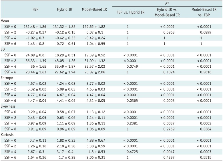
Table 1
Texture Parameters of Pixel Distribution Histogram with/without Filtration on AP (n = 58)
![]()
Table 2
Texture Parameters of Pixel Distribution Histogram with/without Filtration on PVP (n = 58)
![]()
For SD, statistically significant differences between the three reconstruction methods were more frequently observed on AP images. Entropy was demonstrated to be significantly different between the three reconstruction methods on PVP images regardless of the filter values. The difference in skewness and kurtosis between the three reconstruction methods was significant at filter values of 0 and 2 for both phases. Overall, the differences between the reconstruction techniques showed a tendency to become less frequently significant as filter values increased. As an example, the difference in skewness between FBP and hybrid IR was statistically significant when the filter was 0 and 2, while it was non-significant with medium and coarse filters (SSF = 4, 6) on AP (p < 0.0001 vs. 0.1919, 0.6659) and PVP images (p < 0.0001 vs. 0.2381, 1).
Comparison between Patients with Normal Livers and CLD
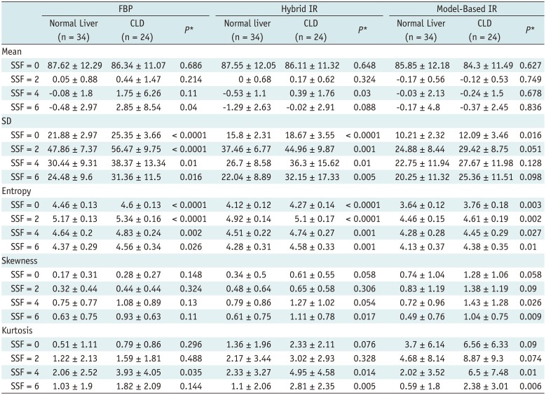
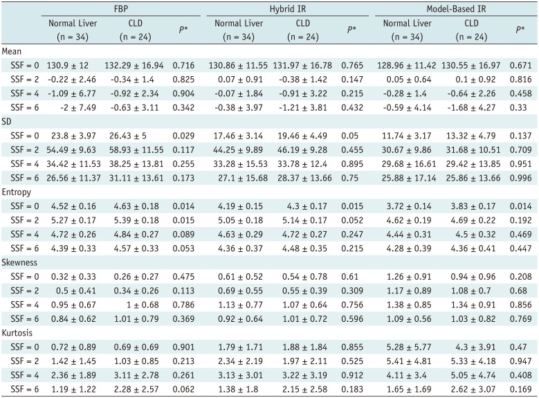
Differences in CT texture parameters between normal livers and CLD are summarized in Tables 3 (AP) and 4 (PVP). Between the two groups, there were more frequent significant differences for AP than PVP images. Among the reconstruction methods, model-based IR showed the least amount of significant differences for both phases. In the PVP images reconstructed with model-based IR, there was no statistically significant difference between the normal liver and CLD groups, except for entropy without filtration (3.72 vs. 3.83, p = 0.014). In addition, the values of texture features showed a tendency to be greater in the CLD group than in the normal liver group for both phases. When the difference between the two groups was statistically significant, the mean value of the texture feature was always greater in the CLD group. As an example, the SD and entropy of AP images reconstructed with FBP were significantly different between the normal liver and CLD groups, with a greater value in the CLD group (p < 0.05) (Fig. 2).
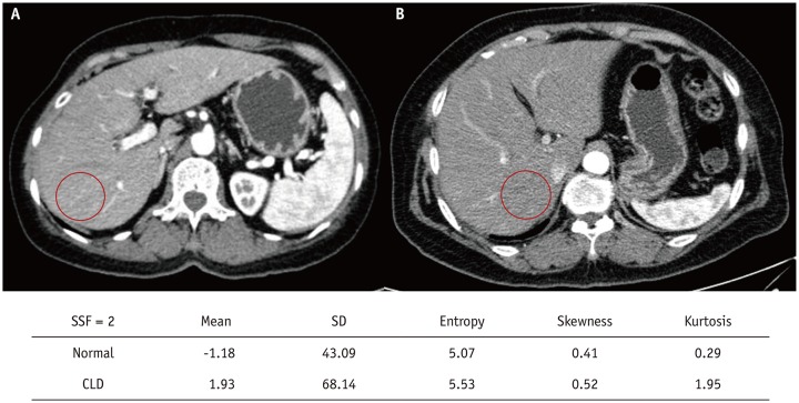 | Fig. 2Examples of normal liver group and CLD group.Arterial phase FBP image from (A) patient in normal liver group and (B) that of CLD patient. Included table shows calculated texture features from each image with filter value of 2. Among them, SD and entropy were greater in CLD patient, which were also demonstrated to be significantly different between two groups (p < 0.0001). CLD = chronic liver disease
|
Table 3
Texture Parameters and p value of Pixel Distribution Histogram with/without Filtration on AP
![]()
Table 4
Texture Parameters and p value of Pixel Distribution Histogram with/without Filtration on PVP
![]()
Inter-Observer and Intra-Observer Reliability Test
Regarding both inter- and intra-observer reliability, ICCs were excellent without filtration (SSF = 0) for both phases. The ICCs of entropy were also always excellent (> 0.75) regardless of the filter values used. Inter-observer ICCs were also excellent for mean and SD, regardless of the filter used. Furthermore, ICCs showed a tendency to become smaller as the filter became coarser, both for inter- and intra-observer reliability (Table 5).
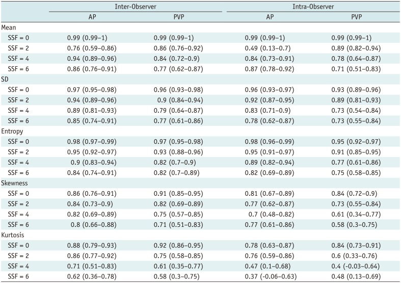
Table 5
Intraclass Correlation Coefficient of FBP image (n = 58)
![]()
Go to :
DISCUSSION
Our study demonstrated that the CTTA features of the liver parenchyma were significantly affected by the reconstruction algorithms used, with model-based IR more frequently showing significant differences in CT texture features compared to the results of FBP or hybrid IR for both phases. This result is in good agreement with previous studies that have investigated the impact of reconstruction methods on CTTA features, focusing on specific lesions (1221). Our results may be explained by the potential alteration of CT features that can occur during the process of noise reduction using hybrid IR and model-based IR techniques compared with FBP. The hybrid IR algorithm first analyzes the projection data as FBP, then applies a model, including photon statistics, to detect very noisy measurements. Thereafter, through an iterative process, the noisy data are penalized while edges are preserved, thereby spatial resolution is preserved with substantial noise reduction (24). However, these extra processes may have also led to differences in texture features between FBP and hybrid IR. Moreover, model-based IR, which does not use FBP data to create the final results (20) but is rather composed of its own unique noise spectrum and tissue depiction pattern (24), showed an even greater significant difference from the other two reconstruction algorithms.
More specifically, the three reconstruction methods examined in our study showed a significant difference in entropy in decreasing order of FBP, hybrid IR, and model-based IR, while for skewness and kurtosis, it was found to be in the opposite order. As IR algorithms directly reduce noise and artifacts resulting from irregularities such as photon starvation, beam hardening, and nonlinearity of individual detector elements (25), it is not surprising that entropy would decrease when an IR algorithm is applied (21). It is also notable that model-based IR exhibited lower entropy than hybrid IR. To the contrary, skewness and kurtosis demonstrated the highest values in the model-based IR image. While reducing noise, model-based IR also acts to smoothen edges; this smudging feature may lead to lesser pixel variability that is reflected in the higher skewness and kurtosis values. In addition to the impact of the reconstruction algorithm itself, the spatial scaling factor was also shown to be a factor influencing CT texture parameters. Our results showed that as the filter became coarser, the significant differences between the three reconstruction methods were less frequent. Considering that the fine filter, which highlights smaller objects, will pick up subtle changes derived from reconstruction algorithms more sensitively than a coarse filter, this result is as expected (26).
We also found that the normal liver group and CLD group demonstrated significant differences in CT texture features more frequently on AP than PVP images. When the difference between the two groups was statistically significant, the mean value of the texture parameter was always higher in the CLD group. These results are as expected considering that CLD has a histologically more heterogeneous parenchyma. As the parenchyma of the liver in CLD has a larger fibrotic component with increased arterial fractions than normal liver parenchyma, the difference between the two groups would be more emphasized on AP images (272829). Furthermore, model-based IR found statistically significant differences between the two groups less frequently than the other methods. We can interpret this result as stemming from the lower capability of model-based IR to reflect subtle heterogeneity in the liver parenchyma in comparison with FBP or hybrid IR, owing to loss of minor image details during its powerful noise reduction (30).
Another notable finding was that the inter- and intra-observer reliability of CTTA was acceptable across all of the various texture parameters. However, ICC tended to become less reliable as the filter became coarser for both inter- and intra-observer reliability. We surmise that this result may be derived from the statistical reason that a higher filter value has a lower number of highlighted units to be used during analysis than a smaller filter value.
Our study has several limitations. First, this is a retrospective study with a limited sample size of 58 patients; therefore, the potential for selection bias cannot be excluded. Second, the CLD group consisted of only 24 patients, and the range of their disease progression status was not evaluated. However, considering that the main focus of our study was on the change and variability of CT texture features according to the use of different reconstruction algorithms, the heterogeneity of our study population should not have affected our main conclusions. Third, our study evaluated the influence of reconstruction algorithms only on first order histogram parameters. As a previous study on PET/CT demonstrated that the standardization of feature extraction methodology is important for second and higher order texture features (31), further analysis of the impact of reconstruction methods on higher order parameters is warranted. Fourth, our study was designed using a single CT machine at a single institution. Thus, investigation of various IR algorithms offered by diverse CT manufacturers with various CT machines for CTTA is warranted in the future.
In conclusion, CT texture features of the liver parenchyma using the filtration-histogram method were significantly affected by the CT reconstruction algorithm used across various filters. Therefore, it is important for CTTA researchers to evaluate the dependency of potential imaging biomarkers on imaging acquisition and reconstruction parameters, as the quality and repeatability of CTTA studies may depend strongly on the consistency of image acquisition and reconstruction method (14). Using unified imaging parameters for CCTA would be an easy and simple solution, but the standardization of feature extraction methodology for CTTA via feature normalization methods, such as voxel size and gray level normalization, could be an alternative approach (32) for more reliable inter-subject comparison and intra-subject longitudinal monitoring.
Go to :
 XML Download