

 PDF
PDF Citation
 Print
Print


In the previous sections, simple linear regression (SLR) 1 and 2, we developed a SLR model and evaluated its predictability. To obtain the best fitted line the intercept and slope were calculated by using the least square method. Predictability of the model was assessed by the proportion of the explained variability among the total variation of the response variable. In this session, we will discuss four basic assumptions of regression models for justification of the estimated regression model and residual analysis to check them.
FITTED REGRESSION LINE AND RANDOM ERROR
Let's recall a bivariate relationship between 2 variables, X and Y, and its depiction of a SLR model in Figure 1A and 1B from the previous section [1]. The expression of the regression model is Y=β0+β1X+ε. The regression model is divided into two parts, the fitted regression line, ‘β0+β1X’ and random error, ‘ε.’ The need of error term is justified by the gap between the line and observed dots because regression line does not go through all the observed values as appeared in Figure 1A.
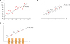 | Figure 1(A) Description of relationship of two variables, X and Y, and error term is expressed as ‘residual’; (B) A single linear regression model; (C) Fitted line and extracted random error part (conceptual).
|
The first part, fitted regression line, is made by connection of the expected means of Y values corresponding with X values such as χ1 to χ5 in Figure 1B. Please find the conceptual distribution of Y, which corresponds with subgroup of χ1, lying on upper vertical direction. The distribution is displayed as a bell-shaped normal distribution with a mean, μy|χ1, at the center. The symbol, μy|χ1 means expected population mean of Y when X variable has the value χ1. In accordance with the previous sections on regression, the expected mean of Y can be symbolized as Ŷ, which is equal to the fitted line, β0+β1X’.
The expected population mean of Y changes from μy|χ1 to μy|χ5 as X changes from χ1 to χ5. The conceptual model suggests that the expected mean of Y can be depicted as the straight line ‘β0+β1X’ by connecting the expected mean of Y matched with subgroups of X. We call the straight line as ‘mean function’ because the expected mean of Y is expressed as the function of ‘β0+β1X’. Please clearly understand that there are numerous means by numerous subgroups of continuous X, and they are linearly connected to make the linear mean function, ‘β0+β1X’. Therefore, we should be able to reasonably assume that the mean function of Y has the form of fitted regression line when we apply the SLR model.
Now let's discuss the second part, random error ‘ε.’ The conceptual form of the random error is depicted as bell-shaped distributions in Figure 1B. At the center of each distribution, there is the expected mean of Y conditioned on each value of X. As the whole model includes both fitted line and random error part, we can get the random error part by subtracting the fitted line, which is the collection of the expected conditional means, e.g., μy|χ1,..., μy|χ5. What would remain after removing the conditional means? Like Figure 1C, after removing means, the mean of difference in all the subgroups will be changed to zero while the shape of distribution will remain unchanged. There will be an identical distribution of random errors with mean of zeros for all the values of X.
Generally, it is reasonable that we assume the shape of random errors as normal distribution because a small amount of errors can occur frequently, while a large amount of errors may be found rarely. Therefore, traditionally, the error terms are assumed as following distributions: ε~N(0,σ2). The equation means that the distribution of errors follows the normal distribution with mean of zero and variance of a constant, σ2. What does the constant variance tell us? The constant variance shows that all the error distribution for all the subgroups have the same variance. In other words, the shape of the error terms is the same for all the subgroups as shown in Figure 1C.
Wrapping up the discussion above, the assumption of fitted line and random error can be collectively summarized into the distribution of Y. Since Y=β0+β1X+ε, the distribution of Y for each subgroup is Y~N(β0+β1X, σ2) for a given X. According to the definition, the distribution of subgroup for the given value of χ1 is a normal distribution with the mean of β0+β1χ1 and with the constant variance of σ2.
How is the error term expressed in the actual data in Figure 1A? The error term is visualized as ‘observed residuals’, which are the distance between the estimated mean of Y (Ŷi) which locates on the line, and the observed value Yi for the ith observation in Figure 1A. An observed residual, ei, is represented as Yi−Ŷi. If the linear regression model is correctly applied to the observed data, the observed errors from the actual data should be in accordance with the assumption on the distribution of random error. In addition, if the fitted line correctly represents the mean response, the means of residuals for all the subgroups should be near zero and the shapes of residual distributions by subgroups follow the assumed normal distribution, similar to the conceptual error distribution in Figure 1C.
The sum and mean of the observed residuals always equal zero. Suppose the mean of observed residuals is a non-zero value. Then, in calculation procedure for coefficients, the nonzero value should be added into the intercept of the fitted line immediately. Similarly, if the slope of observed residuals is nonzero, the relationship should be added into the slope of the regression line. Eventually, the mean of the observed residuals should be zero and also, the line going through the center of residual distribution should be flat with the slope of zero.
FOUR BASIC ASSUMPTIONS AND RESIDUALS
Four basic assumptions of linear regression are linearity, independence, normality, and equality of variance [2]. Only under the condition that the assumptions are satisfied, the estimated linear line can successfully represent the expected mean value of Y variables corresponding to X values. Also if the assumptions are true, the observed residuals should behave in a similar manner. Let's discuss their meanings in detail.
1. Linearity
Linearity means that the means of subpopulation of Y all lie on the same straight line. The scatter plot of X and Y should show a linear tendency. The fitted line of SLR reflects the trend of linearity in the form of linear equation. The error part is expressed as scattered dots around the fitted line as seen in Figure 2A. If the relationship of X and Y is truly a linear one, the scatted dots do not have any trend such as linear, curved, etc., which means that residual and X variable are unrelated. In other words, the residuals appear randomly scattered in relation to X. Also, most observations should lie near the regression line, while observations far away from the line are less frequent, according to the characteristic of assumed normal distribution.
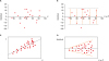
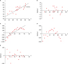 | Figure 2(A) Description of a true linear relationship of two variables, X and Y; (B) Plot of residuals and X from Figure 2A; (C) A mistaken application of linear regression line on squared relationship; (D) Plot of residuals and X from Figure 2C; (E) Plot of residuals and X after adding the true curved relation in the model.
|
Figure 2A and 2B display a linear relationship of X and Y and a scatterplot of residuals for X values. The residuals locate around zero and are randomly scattered without any patterns. The random feature around zero in residual distribution confirms that the assumption of linearity is correct. In contrast, Figure 2C and 2D come from a simulated curved linear relationship. The original relationship is an equation with linear and squared terms:
Figure 2C shows that by mistake, a linear regression is applied on the data, resulting in the first-order linear equation extracted as Ŷ=−644.7+37.8X. After the linear relation is removed as the fitted line, the distribution of residuals in Figure 2D has a clear pattern of second-order curvature. Therefore, we can presume that there is an omitted term of squared-X and also there is a need to add the squared-X term in the model. After adding the squared term, the residuals finally get to be randomly scattered without any trend (Figure 2E).
2. Independence
Independency assumption means that there is no dependency among observations in the data. In other words, outcome of an arbitrarily selected subject does not affect any other outcomes. In traditional statistics, independence among observations was basically assumed, because the simple random sampling procedure guarantees independence of observations. When we collect data only at one-time point, as a cross-sectional data, we do not worry about independence generally. If sample is chosen by a random sampling method and it is a cross-sectional data, we may simply assume independence and do not actually check this further. However, if the sample was selected using cluster sampling method and there are clusters of subjects in the data, we need to consider the dependence in the analysis procedure.
Violation against this independence assumption frequently occurs in most longitudinal data, which is collected repeatedly from the same subject over time. The repeated data tend to correlate with each other. If we observed subjects in time order, we need to plot those against time order (Figure 3A). In many longitudinal data, each successive error may be associated, not independent. We call the phenomenon ‘autocorrelation’. Sometimes the residuals look like cyclic manners between positive and negative error values, which is called ‘snaking plots’ (Figure 3B).
3. Normality
The normality assumption is that the distribution of subpopulation is conceptually normal as shown in Figure 1B. How can we confirm this on the observed residuals? If each error distribution of subpopulation is normal, the collective distribution of residuals should be approximately normal.
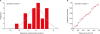
We generally use either histogram of residuals or normal quantile-quantile plot (Q-Q plot) to check the normality of the distribution. As a kind of Q-Q plots, a normal percentile-percentile (P-P) plot may be used. The histogram of residuals should appear similar to normal. In Q-Q plots, the observed points (dots) should be around the diagonal line (Figure 4). Plotting standardized residuals can give us more information to check the size of residuals.

4. Equality of variance
Conceptually, the error terms of all the subgroups are assumed to have the same shape of distribution. That is the normal distribution with mean of zero and variance of a constant, σ2, as shown in Figure 1C. In SLR, we can plot observed residuals against X, because the fitted value and X are linearly related, as shown in Figure 1C. However, in multiple linear regression with more than one X, we need to consider a scatter plot of residuals and fitted values, Ŷ, which is a linear combination of Xs.
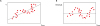
The equal variance assumption means that the degree of spreading or variability of residuals is equal across the subpopulations with different fitted values. We call this feature ‘homoscedasticity,’ which means having the same variance. Figure 5A and 5B do not show any definite violence of the equal variance, because the length of orange dotted lines in Figure 5B are not considerably different. The scattered residual plot against Ŷ displays an approximate squared form around zero.
 | Figure 5Examples of homoscedasticity and heteroscedasticity. (A, B) Residual plot against fitted value of Y (or X) showing homoscedasticity; (C) Relationship of X and Y; (D) Residual plot against fitted value of Y (or X) showing heteroscedasticity.
|
In contrast, Figure 5C and 5D show that the variability is increasing as the value of X or Ŷ increases. We call the phenomenon of unequal variances ‘heteroscedasticity’. As shown in Figure 5C, increasing variability by increase of mean is not a rare phenomenon. For example, let's consider the relationship between income and expenditure. We can easily imagine that the variability of expenditure will increase among people with high income, because they can choose high amount or low amount of expenditure according to their propensity to consume, while poor people can choose only among a limited amount of expenditure because of lack of income. The relationship violates the assumption of homoscedasticity.
As summary, we can use residual plots to check three basic assumptions of linear regression as following:
 XML Download