

 PDF
PDF ePub
ePub Citation
 Print
Print


INTRODUCTION
Scientific journals are means for disseminating scholarly research findings. Journal editors play pivotal roles in this process by maintaining acceptable publication standards. To accomplish their duties, editors need to possess a set of core competencies. Correct presentation of research results is one such competency. Editors often evaluate statistical findings based on tables and graphs in their journal submissions without accessing the raw data. The aim of this article is to reflect on common mistakes in presentation of results that can be detected by skilled editors.
STATISTICAL ANALYSES SECTION
Original articles contain a section, which is presented at the end of the “Methods” to describe in details the employed statistical tests. A note on the software program for statistical analyses should be accompanied by detailed descriptions of how various variables were analyzed and presented. An example of the acceptable note reads as (1):
“The data were … analysed by SPSS version 11.5 for Windows (SPSS Inc., Chicago, IL, USA). … The normality of distribution of continuous variables was tested by one-sample Kolmogorov-Smirnov test. Continuous variables with normal distribution were presented as mean (standard deviation [SD]); non-normal variables were reported as median (interquartile range [IQR]). Means of 2 continuous normally distributed variables were compared by independent samples Student's t test. Mann-Whitney U test and Kruskal-Wallis test were used, respectively, to compare means of 2 and 3 or more groups of variables not normally distributed. The frequencies of categorical variables were compared using Pearson χ2 or Fisher's exact test, when appropriate. A value of P < 0.05 was considered significant.”
PRECISION OF NUMBERS
Some authors report their results with more than enough precision. For example, parts of “Results” of a submitted manuscript may read as “The mean work experience of studied participants was 20.365 (SD, 4.35) years.” Reporting the work experience with 3 digits after the decimal point implies that you measured the variable with an error of ± 4 hours. In fact, the researcher might ask for work experience with an accuracy of no more than a month (2). The values should be presented as “20.4 (SD, 4.4) years” or even “20 (SD, 4) years,” if the authors are about to present the work experience in years (not in months).
The number of decimal places to be reported for common statistics, i.e., the mean, SD, median, and IQR should not exceed that of the precision of the measurement in the raw data (2). Some researchers recommend using one decimal place more than the precision used to measure the variable (3). The same is true for reporting percentages—if a denominator is less than 100, it is unnecessary to report any digits after the decimal point; when the denominator is less than 20, it is better not to report percentages at all. For example, instead of writing “Of 15 patients studied, 26.67% presented with fever,” it is better to write “Four of 15 patients presented with fever.”
In poorly written manuscripts, it is difficult to figure out the denominator. As a rule of thumb, when the value of percentage is higher than the absolute value of the variable, the denominator is less than 100. For example, if in the “Results” section of a manuscript you see “31 (42.47%) of…,” because the value of 42.47 (the percentage) is more than the absolute value of 31, the denominator is less than 100 (it is in fact 73), and the statement should be written as “31 (42%) of…” This rounding off percentages would sometimes cause a difficulty with summing up the percentages to 100%, more prominent in tables. You may encounter situations when the percentages in a table column do not sum up to 100%. As long as calculation of percentages is correct, that minor deviation, “round off error” (at most 1%), is fine and does not need any correction.
REPORTING MEAN, MEDIAN, SD, IQR, STANDARD ERROR OF THE MEAN (SEM), and 95% CONFIDENCE INTERVAL (CI)
Mean and SD are reported to present the center and dispersion of normally distributed data. For non-normally distributed data median and IQR should be reported (4). If distribution of variables is tested, either mean (SD) or median (IQR) is presented. Sometimes information about distribution of parameters is missing. Editors without access to raw data are unable to check the normality. They should, however, know when SD exceeds half of the corresponding mean, it is unlikely that the data follow normal distribution (34). In such cases the results should be presented as median (IQR) with non-parametric tests employed for comparing variables (e.g., Mann-Whitney U and Kruskal-Wallis tests). Student's t test and one-way analysis of variance (ANOVA) are parametric tests.
Authors may report SEM as an index of data dispersion (even with an intention to deceive editors and reviewers, because SEM is always less than SD). Some editors suggest reporting SEM, erroneously considering it a reflection of the dispersion of data in the examined sample or in the population. They should know that SEM reflects the distribution of the mean (4). In fact, 95% CI around the mean is the interval approximately ± 2 × SEM around the mean. Therefore, it is appropriate to report SD to show distribution of data in a sample or a population. Reporting SEM, or 95% CI, is required to demonstrate how accurate is the measurement of the mean. When the sample size is known, SD, SEM, and 95% CI are easily convertible (4).
Confidence intervals, particularly 95% CIs, are increasingly used for reporting estimates of studied parameters in a population. When reporting the prevalence of a disease, it is advisable to additionally report 95% CI. For example, “Twenty-six of 300 studied participants had brucellosis translating to a prevalence of 8.7% (95% CI, 5.5% to 11.9%).” Or, “The mean hemoglobin concentration in men was 3.4 (95% CI, 2.5 to 4.3) g/dL higher than that in women (12.1 [SD, 1.0] g/dL).” The value reported as percentage or mean is in the middle (the arithmetic mean) of the lower and upper limits of 95% CI. In the above examples, 8.7% and 3.4 g/dL are just in the middle of their corresponding 95% CIs—8.7% = (5.5% + 11.9%)/2; and 3.4 = (2.5 + 4.3)/2. This simple rule should always be hold; otherwise, the results are inconsistent.
Authors often report 95% CI for relative risk (RR) and odds ratio (OR) too. For example, it is common to read “Smoking was associated with a higher incidence of lung cancer (OR, 2.6; 95% CI, 1.3 to 5.2).” Here, OR is the geometric mean of the lower and upper limits of the CI, i.e., 2.62 = 1.3 × 5.2. If it is not, then the results are again inconsistent. The same is true for RR.
REPORTING DIAGNOSTIC TEST RESULTS
Authors should be encouraged to report 95% CIs for sensitivity, specificity, positive and negative predictive values, accuracy, and the number needed to misdiagnose in studies of diagnostic tests (56). When receiver operating characteristic (ROC) curve analysis is used, area under the curve, corresponding 95% CI, and criterion for choosing cut-off point should also be presented (789).
ERROR BARS IN GRAPHS
Presenting results in graphs is important. But it is also important to clarify what error bars represent: SD, SEM, 95% CI, or anything else? An example of correct use of error bars is depicted in Fig. 1 (1011). Error bars should be drawn within a valid range only. For example, these cannot be negative when represent 95% CI of a prevalence. Bars with negative values can be reported when variables can take negative values (Fig. 1).
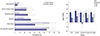 | Fig. 1Examples of correct use of error bars. Left panel: The original legend reads “Prevalence of respiratory symptoms among the garden and factory workers. Error bars represent 95% CI” (10). Note that the error bar for the prevalence of “chest tightness” in “garden workers” is truncated at zero, as a negative prevalence is meaningless. Right panel: The original legend reads “Comparison of the response amplitude (vertical axis) at different frequencies (2–8 kHz [This is the graph for 6 kHz.]) in the study groups receiving various doses of atorvastatin. Error bars represent 95% CI of the mean. N/S stands for normal saline” (11). Note that some of the error bars extend to areas with negative amplitude response, as unlike the prevalence, a negative amplitude response does make sense (re-used with permission in accordance with the terms of the Creative Commons Attribution-NonCommercial 4.0 International License).
CI = confidence interval, N/S = normal saline, TTS = temporary threshold shift, PTS = permanent threshold shift.
|
UNITS OF MEASUREMENT
Another important issue is correct presentation of units of measurements (12). As an example, in a manuscript submitted to a transplantation journal, we read “Serum tacrolimus level was 6.18.” The missing unit of measurement is “µg/L.” Too often such omissions take place in figure axes, tables, etc. Authors who are experts in their fields do not mention the units of measurements in their daily work and during professional meetings. They should, however, be advised to always present the units of measurements in their articles because scholarly journals employ various standards for units. Most but not all journals use the international system of units (SI). Knowing which units are presented is essential for correct secondary analyses of the data to avoid mixing oranges and apples.
REPORTING P VALUE
The P value is by far the most commonly reported statistics. Editorial policies of reporting P values differ. Some journals use the well-known arbitrarily chosen threshold of 0.05 and report P values as either “P < 0.05” or “non-significant.” Most experts suggest reporting the exact P value. For example, instead of “P < 0.05,” it is suggested reporting “P = 0.032” (313).
In biomedical research, it is rarely necessary to report more than 3 digits after the decimal point. Presenting “P = 0.0234” is therefore inappropriate whereas “P = 0.023” is better. Sometimes a highly significant P value is mistakenly reported as “P = 0.000” (e.g., for “P = 0.0000123”). In such cases, the value should be reported as “P < 0.001” (4).
P values should only be reported when a hypothesis is tested. Believing in that reporting significant P values are important for positive editorial decisions, authors without a clear hypothesis inappropriately report several P values to dress up their manuscript and make them look scientific. For example, part of “Results” in a submitted manuscript reads “Mean age of patients with wheezing 11.6 months (P = 0.001).” But it is unclear whether any hypothesis is tested.
Often it is better to report 95% CIs instead of P values. For example, it is advisable to report “Smoking was associated with a higher incidence of lung cancer (OR, 2.6; 95% CI, 1.3 to 5.2).” instead of “Smoking was significantly (P = 0.04) associated with a higher incidence of lung cancer (OR, 2.6).” Reporting both P value and 95% CI is no more informative than reporting only 95% CI. While P value only indicates if the observed effect is significant or not, 95% CI additionally delineates the magnitude of the effect (i.e., the effect size). Editors can omit a P value when the corresponding 95% CI is reported, as the latter is more informative.
Even though it seems obvious, many researchers, even statisticians and epidemiologists, have variable interpretations of P values (14). Considering the well-established threshold of 0.05, a P = 0.049 is considered statistically significant, while a P = 0.051 is not. This results in coining some interesting terms including “partially significant” or “marginally significant” used by some authors and interpreting the non-significant results (with a P = 0.06, for example) in the manuscript “Discussion” section in a way if the difference is in fact significant. If we accept to use the set cut-off value of 0.05, we should abide to it and consider all results with a P value equal to or more than 0.05 non-significant and interpret that based on observed data, there are no evidence to support that the observed effect likely exists in the population (and it likely results from sampling error), and not discuss the observed effect. Interpretations by representatives of the dominant school of statistics, the so-called frequentist statistics, may differ from those by representatives of Bayesian statistics (1516). For example, frequentist statistics tests if the null/alternative hypothesis can be rejected or accepted, considering the data collected from a representative sample (using a pre-defined cut-off of say 0.05 for P value). Bayesian statistics gives the post-test probability (odds) of a hypothesis being true, based on the pre-test probability (odds) of the hypothesis and the collected data. No hypothesis is rejected or accepted. And what researchers have is only a change in likelihoods, which seems more natural. Researchers investigate available evidence to report increased or decreased probability of a hypothesis.
I believe associations of science editors should encourage journal editors to promote the use of Bayesian statistics while under- and postgraduate students should be trained in employing Bayesian techniques.
KAPLAN-MEIER SURVIVAL ANALYSIS
Cox proportional hazards model is widely used in biomedical research to estimate the hazard rate of developing an outcome of interest given an exposure of interest and after adjusting for known confounding variables. One of the main presumptions in the analysis is the “assumption of proportionality,” which is often ignored and not checked. Crossing survival curves in a Kaplan-Meier survival graph (17) means that it is highly likely that such an assumption is violated and the results of the analysis are unreliable (Fig. 2). In such cases, other statistical methods could be used for proper data analysis (18).
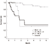 | Fig. 2Part of a panel of Kaplan-Meier survival curves (17). Note the dotted curve crossing other 2 curves. This clearly violates the “proportional hazard” assumption made in Cox proportional hazards model (re-used with permission in accordance with the terms of the Creative Commons Attribution Non-Commercial License [http://creativecommons.org/licenses/by-nc/3.0/]).
MELD = model for end-stage liver disease.
|
CONCLUSION
Journal editors have an important role in correcting the flow of scientific research results. While not having access to the raw data, they should rely on clues in the manuscripts, indicating erroneous presentation of the data. To pick concealed errors, editors should look for inconsistencies, which are eye-balling for non-experts in statistics. Associations of journal editors may improve research reporting by arranging trainings on basic statistics and research methodology to help their members correct statistical reporting during the manuscript triage, save the reviewers' precious time, and eventually safeguard the body of scientific evidence.
 XML Download