

 PDF
PDF Citation
 Print
Print


In the previous section, we established a simple linear regression line by finding the slope and intercept using the least square method as: Ŷ=30.79 + 0.71X. Finding the regression line was a mathematical procedure. After that we need to evaluate the usefulness or effectiveness of the regression line, whether the regression model helps explain the variability of the dependent variable. Also, statistical inference of the regression line is required to make a conclusion at the population level, because practically, we work with a sample, which is a small part of population. Basic assumption of sampling method is simple random sampling.
USEFULLNESS OF REGRESSION LINE
Coefficient of determination (R-square)
An important purpose of data analysis is to explain the variability in a dependent variable, Y. To compare models, we consider a basic situation where we have information on the dependent variable only. In this situation, we need to model the mean of Y, Ȳ, to explain the variability, which is regarded as a basic or baseline model. However, when we have other information related to the dependent variable, such as a continuous independent variable, X, we can try to reduce the (unexplained) variability of dependent variable by adding X to the model and we model a linear regression line formed by the predicted value by X, Ŷ. Hopefully, we can expect an effective reduction of variability of Y as the result of adding X into the model. Therefore, there is a need for evaluation of the regression line, such as “how much better it is than the baseline model using only the mean of the dependent variable”.
Figure 1 depicts baseline and regression models and their difference in variability. The baseline model (Figure 1A) explains Y using only the mean of Y, which makes a flat line (Ȳ). The variability in the baseline model is the residual ① Y − Ȳ. In Figure 1B, X, which has a linear relationship with Y, is introduced as an explanatory variable and a linear regression line is fitted. In the regression model, residual ② Y − Ŷ is reduced compared to ①. The explained variability ③ Ŷ − Ȳ represents the amount of reduced variability of Y due to adopting regression line instead of mean Y.
Figure 1
Depiction of comparative models: (A) a baseline model with mean of Y and its residuals (① Y − Ȳ, total variability); (B) fitted regression line using X and residuals (② Y − Ŷ, remaining residual); (C) the residual ① in (A) was divided into the explained variability by the line (③ Ŷ − Ȳ, explained variability due to regression) and reduced but remaining unexplained residual (②).
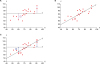
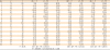
Table 1 shows the same three quantities ① Y − Ȳ, ② Y − Ŷ, and ③ Ŷ − Ȳ, which appear in Figure 1. Ȳ represents mean of Y and Ŷ, the predicted value of Y by the regression equation Ŷ = 30.79 + 0.71X, which are points on the regression line. To quantify the effect of the regression model, we may use a form of ratio of ① Y − Ȳ and ③ Ŷ − Ȳ. To facilitate the calculation procedure, we practically use squared sum, such as ∑(Y − Ȳ)2 and ∑(Ŷ − Ȳ)2. For the baseline model, we square all the residuals ① Y − Ȳ and sum them up, which is called sum of squares of total (SST), ∑(Y − Ȳ)2. SST is the maximum sum of squares of errors for the data because the minimum information of Y itself was only used for the baseline model. For the regression model, we square all the differences ③ Ŷ − Ȳ and sum them up, which is called sum of squares due to regression (SSR), ∑(Ŷ − Ȳ)2. SSR is the additional amount of explained variability in Y due to the regression model compared to the baseline model. The difference between SST and SSR is remaining unexplained variability of Y after adopting the regression model, which is called as sum of squares of errors (SSE). SSE can be directly obtained by sum of squares of residual, ∑(Y − Ŷ)2.
Table 1
Calculation of sum of squares of total (SST), sum of squares due to regression (SSR), sum of squares of errors (SSE), and R-square, which is the proportion of explained variability (SSR) among total variability (SST)
If the regression line is flat as in Figure 1A, there is no contribution of X. Therefore, regression line will be of no use in explaining Y in this case. Larger absolute values of Ŷ − Ȳ mean larger contribution of the regression line. To quantify the contribution of the regression line, we use ratio of SSR and SST. We call the ratio as R-square, which is also called ‘coefficient of determination’. The coefficient of determination is interpreted as the proportion of additional explanation of variability in the regression model among the total variability. The proportion, R-square, is also frequently expressed as a percentage. As below, we can conclude 53.8% of SST is explained by the estimated regression line to predict the dependent variable.
 .
.We use the term ‘fit’ which indicates whether or not the model fits well with the observed data. In this case, the regression model using X fits well because it explains a big amount of variability among SST. A large R-square value represents a good fit.
Overall F test: a global evaluation of model
As mentioned above, SST is divided into SSR and SSE. A relatively small SSE can be interpreted as a “good fit” of the model. The usefulness of the regression model is tested using F test as a global evaluation of the regression model. In the F test, F value is defined as the ratio of mean of squares of regression (MSR) and mean of squares of error (MSE), which are under the title of ‘Mean squares’ in Table 2. Mean squares are defined as the means of SSR or SSE per one degree of freedom (df) and are obtained by dividing SSR or SSE by their own df as shown in Table 2. A large F value represents relatively large MSR and relatively small MSE, which can be interpreted as a good contribution of the regression model. A large F value leads to the rejection of null hypothesis that all the slopes are zero. If all the slopes are zero, the regression line is useless because it is identical to the simple mean of Y, such that Ŷ = Ȳ.
Table 2
A general form of analysis of variance table for the global evaluation of the regression line

| Source | Sum of squares | df | Mean squares | F |
|---|---|---|---|---|
| Regression | SSR = ∑(Ŷ − Y̅)2 | p | MSR = SSR/p | MSR/MSE |
| Residual | SSE = ∑(Y − Ŷ)2 | n − p − 1 | MSE = SSE/(n − p − 1) | |
| Total | SST = ∑(Y − Y̅)2 | n − 1 |
The formal expression of the overall test is as follows:
Test statistic: F = MSR/MSE
Table 3 shows the analysis of variance table for the example data. The F value is calculated as follows:
Table 3
An analysis of variance (ANOVA) table for the example data

| ANOVA | |||||
|---|---|---|---|---|---|
| Model | Sum of squares | df | Mean square | F | p value |
| Regression | 1,475.036 | 1 | 1,475.036 | 20.947 | <0.001 |
| Residual | 1,267.514 | 18 | 70.417 | ||
| Total | 2,742.550 | 19 | |||
Table was cited from appendix of reference [1] which has modified as table format.
df, degree of freedom.
To get p values corresponding to the calculated F values, we can refer to a website named ‘p-value from F-ratio Calculator’ at http://www.socscistatistics.com/pvalues/fdistribution.aspx. We provide ‘F-ratio value’ as 20.947, ‘df-numerator (df of MSR)’ as 1, and ‘df-denominator (df of MSE)’ as 18 in Table 3. Then finally, we get the p value as 0.000234, which can be expressed as p < 0.001, as well. We reject null hypothesis that the regression model is useless and conclude that there is at least one non-zero slope, which means the regression model is contributing in reduction of error.
EVALUATION OF INDIVIDUAL SLOPE(S)
T test: test on significance of slope
If the global evaluation of the regression model concludes there is at least one nonzero slope, we want to know which slope is nonzero and its estimated size. In simple linear regression with only one X, the result of global F test and the significance of the slope share the same conclusion. When we have a simple linear regression model such as Y = b0 + b1X + e (residual), the formal test on the significance of slope is as follows:
Test statistic: , where seb1 is the standard error of b1.
, where seb1 is the standard error of b1.This test is asking whether a statistically significant linear relationship exists between the dependent and independent variables. If the answer is no, the regression model is no good because the basic assumption was a linear relationship between two variables. If there is no linear relationship, the slope is near zero and the scatterplot of Y and X is expected to show a random scatter, which means there is no correlation.
Table 4 displays information on regression coefficients from the example data from the previous section [1]. Information on slope is in the line of X. The point estimate b1 is 0.712 and its standard error (seb1) is 0.155. The standard error of b1 (seb1) and test statistic are obtained as follows.
Table 4
Regression coefficients from the example data

Table was cited from appendix of reference [1] which has modified as table format.
SE, standard error; CI, confidence interval.

 p < 0.001
To get p values corresponding to the calculated t values, we can refer to a website named ‘p value from T score calculator’ at http://www.socscistatistics.com/pvalues/tdistribution.aspx. We provide ‘T score’ as 4.577, and ‘DF’ as 18, which is df of MSE, n-2, and then finally we get the p value as 0.000234, which is the same p value from F test above. We reject null hypothesis that the slope is zero and conclude that there is a significant linear relationship between Y and X.
95% confidence interval (CI) of slope
As a statistical inference procedure, we usually use an interval estimation procedure. We got the estimate using a sample. But if we take different sample from the population, we may have different estimate. The phenomenon is called ‘sampling variability’. Therefore, we usually make CI in which we believe the parameter β1 is included with certain degree of confidence.
The 95% CI of β1 is expressed as b1 ± tdf=18,0.025 * seb1. We already know b1 and seb1, shown in Table 4. We can get the critical t value with df = 18 from a website ‘Free critical t value calculator’ at https://www.danielsoper.com/statcalc/calculator.aspx?id=10. We provide ‘Degrees of freedom’ as 18, ‘Probability level’ as 0.05, and get t value (2-tailed) as 2.100. We are ready to construct the 95% CI of β1 as follows:
Does the interval contain zero? No! Therefore, we can conclude that the slope of X is nonzero similar to the result from the t test above.
 XML Download