Introduction
The characterization of drug elimination kinetic studies is an essential part of the development process, and it requires accurate and precise estimation of the parameters of the relevant kinetic models. Michaelis-Menten kinetics is one of the bestknown models of enzyme kinetics in
in vitro drug elimination or drug-drug interaction experiments. The Michaelis-Menten equation (M-M equation) consists of two parameters, the maximum reaction rate (V
max) and the Michaelis constant (K
m) describing the rate of enzymatic reactions by relating reaction rate (V) to the concentration of a substrate ([S]).[
1] By definition, Km is equal to the concentration of the substrate at half V
max. It can also be thought of as a measure of how well a substrate complexes with a given enzyme, otherwise known as its binding affinity. An equation with a low Km value indicates a large binding affinity, as the reaction will approach V
max more rapidly. An equation with a high Km indicates that the enzyme does not bind as efficiently with the substrate, and Vmax will only be reached if the substrate concentration is high enough to saturate the enzyme. Therefore, K
m is an intrinsic parameter of enzyme-catalyzed reactions and it is significant for its biological functions.[
2]
Two most commonly used methods for determining the parameters of the M-M equation are the Lineweaver-Burk plot and the Eadie-Hofstee plot, both of which are linearization methods transforming the original nonlinear M-M equation into a linear one, and the data is then fit by a linear regression, which can be displayed as a straight line in 2-dimensional graph. In spite of the simplicity and familiarity of linear regression method, these approaches have some pitfalls. The most common problem with these transformations is the fact that transformed data does not usually satisfy the basic assumptions of linear regression, that is, the distribution of data around the straight regression line follows a Gaussian distribution, and the standard deviation of the distribution is equal at each value of the independent variables. For this reason, there has been increased interest in fitting full time course kinetic data to nonlinear equations based on numerical integration of rate equations without linearization.[
345]
Simulation studies are useful for comparing various estimation methods using virtual in vitro enzyme kinetic data. In this study, we compared the accuracy and precision of parameter estimation for the M-M equation determined by various estimation methods, including traditional linearizing methods and nonlinear regression methods.
Go to :

Methods
Simulation Data Generation
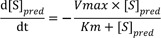
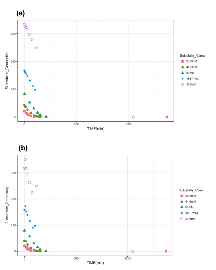
Invertase is the enzyme which catalyzes the reaction which results in the inversion of optical rotation from positive for sucrose to net negative for the sum of fructose plus glucose. Based on the M-M equation and the studied kinetics of invertase (V
max=0.76 mM/min and K
m=16.7 mM), a set of virtual substrate concentration ([S]) data without considering residual errors was simulated for 5 initial substrate concentrations of 20.8, 41.6, 83, 1667.7, and 333 mM and at pre-specified times thereafter using the deSolve package in R 3.3.3.[
1]
where [S]pred is the predicted substrate concentration without error.
The observation time points for each concentration in the simulation were as follows; 0, 17, 27, 38, 62, 95, and 1372 min for initial concentrations of 20.8 mM; 0, 10, 30, 61, 90, 112, 132, and 154 min for 41.6 mM; 0, 50, 90, 125, 151, and 208 min for 83 mM; 0, 8, 16, 28, 52, 82, and 103 min for 166.7 mM; and finally 0, 7,14, 26, 49, 75, 117, and 1052 min for 333 mM.
A set of final virtual experimental data was constructed from the error-free data set by incorporating an additive error model or a combined (additive + proportional) error model.
Additive error model: [S]i = [S]pred + ϵ1i
Combined error model: [S]i = [S]pred + ϵ1i + [S]pred × ϵ2i
where [S]pred is an error free-substrate concentration calculated from the M-M equation, [S] is an error incorporating substrate concentration, ϵ1 is a random variable following a normal distribution with a mean of 0 and a standard deviation of 0.04 (calculated as approximately half of the lowest value of [S]pred), ϵ2 is a random variable following a normal distribution with mean of 0 and standard deviation of 0.1 (an arbitrarily selected high value), and i is the index of simulation replicates.
A Monte-Carlo simulation with 1,000 replicates for each scenario was carried out using R
M-M Parameter Estimation by Various Estimation Methods and Analysis of the Estimation Results
The V
max and K
m values were estimated from the original simulation dataset or the manipulated simulation data using the following 5 different estimation methods, which are summarized in
Table 1.
Table 1
Summary of estimation methods
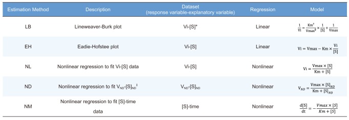
|
Estimation Method |
Description |
Dataset (response variable-explanatory variable) |
Regression |
Model |
|
LB |
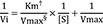
Lineweaver-Burk plot |
Vi-[S]*
|
Linear |
|
|
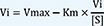
EH |
Eadie-Hofstee plot |
Vi-[S] |
Linear |
|
|
NL |
Nonlinear regression to fit Vi-[S] data |
Vi-[S] |
Nonlinear |
|
|
ND |
Nonlinear regression to fit VND-[S]ND‡
|
VND-[S]ND
|
Nonlinear |
|
|
NM |
Nonlinear regression to fit [S]-time data |
[S]-time |
Nonlinear |
|

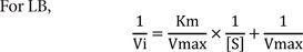
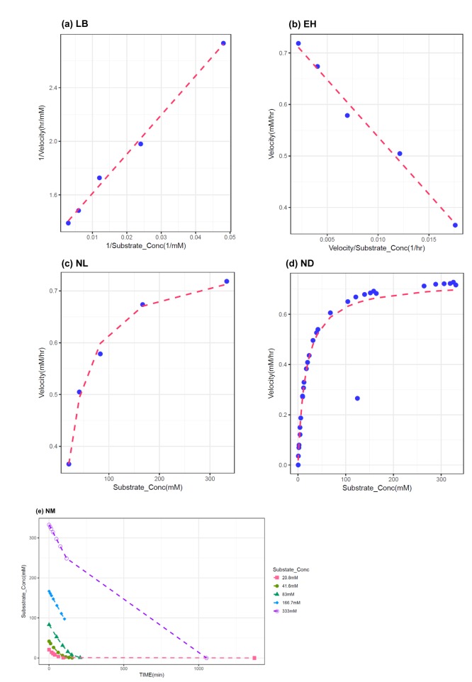
1) Lineweaver-Burk plot (LB)
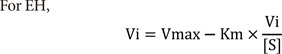
2) Eadie-Hofstee plot (EH)
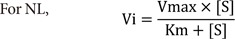
3) Nonlinear regression to fit Vi-[S] data (NL), where Vi is the initial velocity.
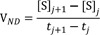
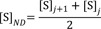
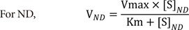
4) Nonlinear regression to fit VND-[S]ND (ND), where VND is the velocity calculated by the average rate of change for the substrate concentrations ([S]) at adjacent time points and [S]ND is the corresponding substrate concentrations to VND calculated from the averaged substrate concentrations ([S]) of adjacent time points.
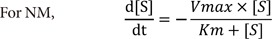
5) Nonlinear regression to fit [S]-time data (NM)
A dataset suitable for each estimation method was prepared from the original simulated dataset as follows.
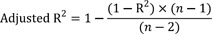
For the estimation methods using initial velocity, i.e. LB, EH, and NL, Vi values were calculated from the original simulated substrate concentration versus time ([S]-time) data using linear regression in R. For each [S], regressions were repeated using the first 3 points, then the first 4 points, and the first 5 points, etc. and the adjusted R2 was computed as follows:
where n is the number of data points in the regression and R2 is the square of the correlation coefficient, respectively. The slope calculated from the regression with the largest adjusted R2 value was selected. However, if the adjusted R2 did not improve, but was within 0.0001 of the largest adjusted R2 value, the regression with the larger number of points was used. The slope was then transformed to a positive value to indicate the velocity of the reaction product as follows:
For LB and EH, additional manipulation was performed after the Vi values were obtained. For LB, the reciprocal of Vi and [S] was taken and 1/Vi versus 1/[S] data was produced. For EH, Vi/[S] was computed and Vi versus Vi/[S] data was created.
For ND, a velocity (VND) (was computed from the average rate of change of [S] for adjacent time points and the corresponding substrate concentration ([S]ND) (was obtained averaging the substrate concentrations ([S]) of adjacent time points.
where is the index of time points.
For NM, the original simulation dataset by itself was used with no data manipulation.
After manipulating a dataset to a suitable form for each estimation method, estimation was conducted by first order conditional estimation with interactions in NONMEM (version 7.3, ICON Development Solutions, Ellicott City, MD, USA). The models for each analysis methods were as follows and the residual variabilities were applied according to the error model used for the simulation.
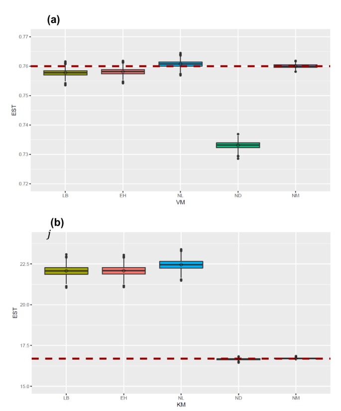
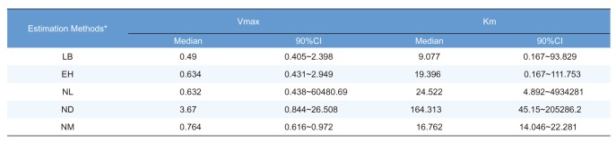
The median estimated values and 90% confidence intervals (CIs) of Vmax and Km for a particular fitting method were subsequently calculated for the purposes of comparison.
Go to :
Discussion
Undoubtedly, the M-M theory is the foundation upon which most current quantitative analysis of enzymes is built.[
6] Advances have been made which describe more complex behavior, such as allosteric regulation or cooperativity in the framework of the M-M theory or outside it, but the basic model is still widely used for most single-substrate enzyme kinetics. The classical approach to deriving the parameters of M-M, i.e.,V
max and K
m, is through initial-rate measurements. Under the quasisteady state approximation, the M-M equation and corresponding nonlinear differential equations collapse into a single hyperbolic function. The initial stages of an array of experiments can describe this relation between reaction speed and substrate concentration. This yields the maximal reaction rate, V
max, and Michaelis constant, K
m, which corresponds to the substrate concentration at half of V
max.[
7] Unfortunately, an accurate estimation requires a large amount of data as well as substrate concentrations much higher than K
m, which are often difficult to obtain. Thus, there is great value in directly determining the M-M constants from the [S]-time curve.[
8] Here, we have conducted a simulation study to see if direct nonlinear fitting method is reliable compared to the classical approach or some other methods derived from the classical approach.
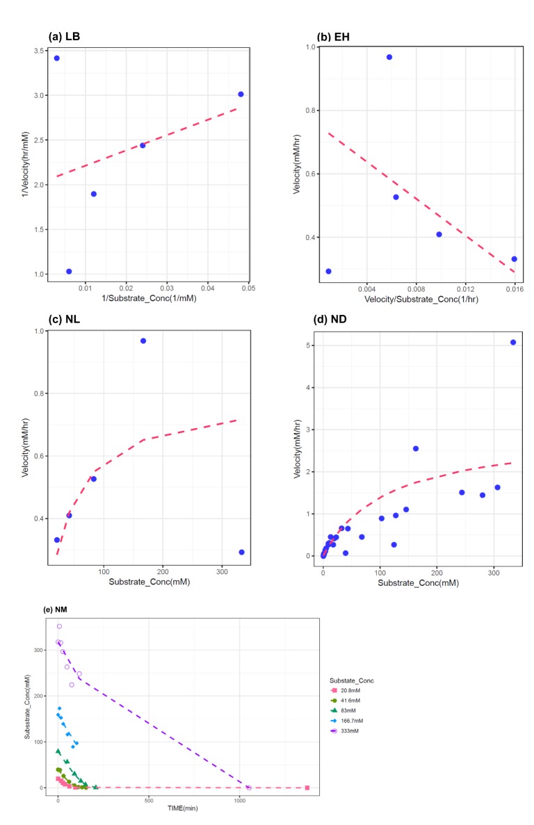
In this study, 1000 replicates of simulation data were generated based on the original M-M data with assay errors according to 2 different residual error models. The simulation data were fitted by 5 different methods which consisted of 1 nonlinear direct fitting method for [S]-time data (NM) and 4 linear or nonlinear fitting method for transformed V-[S] data (LB, EH, NL, ND).
During data generation process, we incorporated additive error or combined error model as the residual error model into the simulation data. This is because these two models generally reflect the assay errors arising from pharmacokinetic and pharmacodynamic data and the errors originating from model misspecification of experiment data. For dense pharmacokinetic data, the combined error model broadly reflects assay errors, whereas for pharmacodynamic data, additive error model may be sufficient. Exponential and proportional models are generally avoided because of the tendency to overweight low concentrations.
In posthoc analysis, estimates obtained with minimization failure as well as those with successful minimization were used. The causes of all failures were rounding errors associated with SIGDIGIT of NONMEM. Software programs other than NONMEM usually judge minimization success or failure regardless of SIGDIGIT. SIGDIGIT of NONMEM is calculated in the scaled and transformed parameter (STP) space and there are usually more actual significant digits in the original scale.[
9] Additionally, the median values and 90% CI for the parameters estimated from the only minimization successful data were almost same as those of the parameters estimated from the whole data set including rounding errors. Considering this, estimates obtained from NONMEM runs with minimization failure due to rounding error seems to be reasonable.
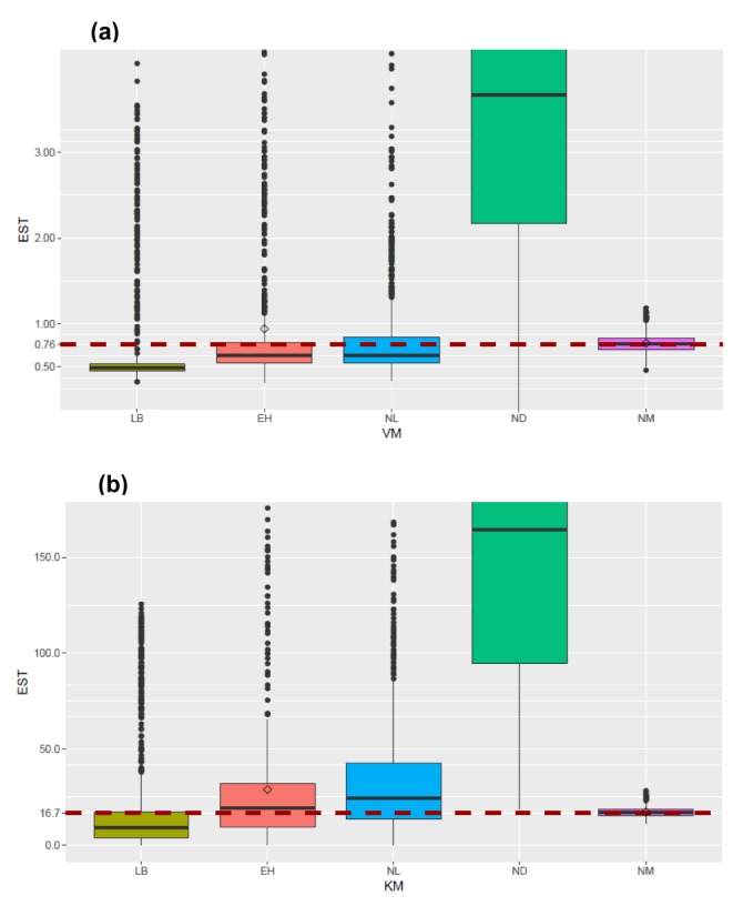
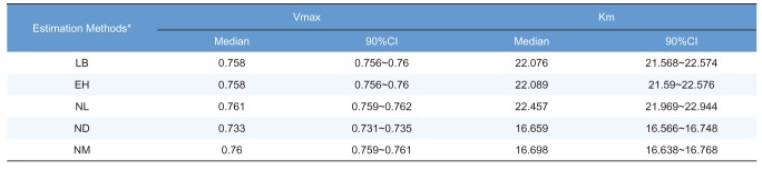
When comparing the median values and 90% CI of the parameters estimated from each fitting method, estimation by NM was the most accurate and precise among the 5 methods, for both error models. That is, the use of nonlinear regression and untransformed data yielded the most reliable estimation of enzyme kinetic parameters. In particular, the superiority of parameter estimation of nonlinear regression directly to [S]-time data was clearly revealed in the simulated data incorporating combined error. When a combined error was applied, NM method performed fairly well and gave comparable answer to those of the simulation data incorporating additive error, especially for point estimates, whereas the other methods gave considerably poorer answers. In the combined error model, % CV (coefficient of variation) is the greatest at the lowest concentration and decreases with the increment of concentration. In the
in vitro experiments conducted at low initial concentration with larger assay variability, the difference of biases in the parameter estimation between NM method and the other method can be maximized, because NM method uses dense, serial concentration over time data, providing relatively unbiased estimates, whereas the other methods uses only one or few velocity data, resulting in more biased estimates (as shown in
Figure 3). The combined error can represent complex scenarios in which experimental errors such as variation in the measured volume of substrates and enzymes, variations during substrate dilution and imprecisions in the instrumentation are mixed. Although this level of error was higher than is likely in practice, the differences between the 5 methods are seen most clearly using this error model. In addition to reliable estimation, NM bypasses the need to subsequently fit the concentration dependence of the measured rate after fitting the primary kinetic data ([S]-time) to a simplified function, which is the process performed for the other methods.
It was apparent from this study that the ND method gave answers that were the least accurate and generally imprecise. The unreliable estimation of ND method can partly explained by the unequal variance of velocity and the correlated error between velocities induced by the unequal time intervals of the simulation data.
When comparing the linear transformation methods (LB and EH) using linearized Vi-[S] data, EH plots and LB plots gave similarly reliable answers in the additive error model but the EH plot exhibited more accurate and similarly precise estimation in the combined error model, which was consistent with previous investigations.[
10] The LB plot has the disadvantage of compressing data points at high substrate concentrations into a small region and emphasizing the points at lower substrate concentrations, which may alter the slope of the line due to the long lever arm effect of the reciprocal plot, leading to a poor estimation of Vmax and Km in the combined error model.[
7] On the other hand, the EH plot bypasses the unequal weighting of errors in the reciprocal plot, an implicit fault of LB plot, because it does not use a reciprocal plot and separates the two kinetic parameters, V
max/K
m and V
max as 1/slope and intercept, respectively, thus giving more reliable answers than the LB plot. Although the EH plot produces more reliable estimates, the presence of the dependent variable, velocity, on both axes makes rigorous error analysis difficult. In all linear transformation methods, linear regression was used to estimate the slope and intercept of the straight line, and afterwards V
max and K
m were calculated from the straight line parameters. Although these methods are very useful for data visualization and are still widely employed in enzyme kinetic studies, linear transformation makes them prone to errors, as shown in this study.
When comparing the linear transformation methods (LB and EH) and the nonlinear regression method using transformed Vi-[S] data (NL), NL generally gave similarly accurate but poorer answers than LB and EH, especially in the combined error model. This is likely to be result of the bias caused by transformation from [S]-time to Vi-[S] in which the only first 10-20% of the reaction data was used, although NL is more suitable for fitting to Vi-[S] data itself.
For nonlinear regression, we used NONMEM, the estimation method of which is based on maximum likelihood estimation (MLE) and STP whereas other software packages usually used in enzyme kinetics, such as Excel and GraphPrism, perform fitting based on least square estimation (LSE) and original scaled and untransformed parameters.[
1112] The latter require a good initial guess of parameters and there is no guarantee of convergence to the global minimum.[
1314] The former is generally insensitive to initial values and reaches the global minimum in our experience. Thus, although we did not intensively compare NONMEM-like estimation software and the other software in this study, we recommend using NONMEM-like estimation software for nonlinear regression.
In conclusion, estimating the actual parameters of the M-M equation from data is the aspiration of all researchers involved in enzyme kinetics research. This remains to be perfected though various estimation methods have been used. In this study, the superiority of direct nonlinear regression to [S]-time data was clearly revealed through comparing the accuracy and precision of the parameters of the M-M equation, as determined by various estimation methods from the simulated data, especially simulated data incorporating combined error, which might represent complex experimental situations. Our results suggest that direct nonlinear fitting of [S]-time data using program such as NONMEM can provide a better parameter estimation with regard to accuracy and precision in enzyme kinetics, which is the basis of in vitro drug-drug interaction study.
Go to :


 PDF
PDF ePub
ePub Citation
 Print
Print


 XML Download