

 PDF
PDF ePub
ePub Citation
 Print
Print


In the previous section, we discussed risk and odds. Both risk and odds can be applied to a cohort study designs based on population. On the other hand, a case-control study is not based on population but designed by separate sampling procedures in the disease group and no disease group. Therefore, there is no denominator to estimate the risk in the entire population and only odds can be obtained in the case-control design. Regarding those study designs, we'll talk about definitions, applicability, difference, and interpretation of risk difference (RD), risk ratio (RR), and odds ratio (OR) as measures of effects in studies with cohort and case-control design.
Definition
1. Risk difference (RD), attributable risk (AR), excessive risk
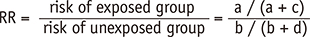
RD or AR is defined as the difference in risk of a condition such as a disease between an exposed group and an unexposed group (Table 1).

Risk difference, risk ratio, and odds ratio as measures of effects in cohort design
A cohort study design pursues the effect of exposure such as treatment, prospectively. In the cohort study, we extract an adequate size of a random sample from the target population, then randomly assign the subjects into either the expose group or unexposed group. The effect of exposure is observed as the changes in outcome of interest over time. Risk is easily calculated as the number of persons having the disease in exposed and unexposed groups divided by the number of all the persons in both groups. In the cohort study, we have a clear denominator: the number of persons assigned in the groups. RD and RR are frequently used to assess the association between the exposed and control groups. RD, which is also known as AR or excessive risk, represents the amount of risk, which decreased or increased when the exposure exists compared to that when the exposure is absent. A positive RD value means increased risk and a negative one means decreased risk by the exposure. RR is calculated as the risk of an exposed group divided by the risk of an unexposed group. A RR value of 1 means no difference in risk between groups, and larger or smaller values mean increased or decreased risk in an exposed group compared to the risk in an unexposed group, which can be interpreted that the occurrence of disease is more or less likely in the exposed group, respectively.
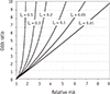
In addition, we can also use OR for the same purpose in cohort studies. OR is the ratio of odds of disease in an exposed group and an unexposed group. The interpretation OR is not as intuitive as RR. An OR value of 1 means no difference in odds between groups, and larger value than 1 means increased odds in exposed group, interpreted as a positive association between having disease and having exposure. Contrarily an OR value of smaller than 1 means decreased odds in exposed group which is interpreted as the association between having disease and not having exposure. Though the interpretation of OR is similar to that of RR, they have similar values only when risks of both groups are very low, e.g., p < 0.1. Otherwise, they show different values. As seen in Table 2, the values of RR and OR are approximately the same only when risk of both groups are very low (p < 0.1, Examples 1 - 5 in Table 2). However, when risks of either one or both groups are not very low (p > 0.1), there are considerable discrepancy between RR and OR values (Examples 6 - 14, Table 2). A general rule is that a value of OR is always reflecting larger effect size or stronger association, by showing smaller OR values than corresponding RR values when RR < 1 and larger OR values when RR > 1. In Table 2, we can confirm that all the cases with RR larger than 1 had much larger OR values (Examples 6 - 8 and 10 - 14), and a case with RR smaller than 1 had a smaller OR value than the corresponding RR value (Example 9). Therefore, incorrect interpretation of OR value as RR will lead to an overstatement of the effect by either erroneously increasing or decreasing the true risks. Figure 1 depicts that the differences between OR and RR values get larger as the levels of baseline risk in the control group (I0) increase.1 Especially when baseline risk is as large as 0.5, the maximum RR value is confined to 2, while OR value approaches infinity.
OR has been used as a very popular estimate of effect in epidemiological studies. As the logistic regression has been frequently used in multivariate assessment of binary outcomes, OR which is the exponentiated regression coefficient from logistic regression has been popular, too. The logistic regression has a computational advantage that the convergence is efficient because the related logit link can convert risk (p) values, confined from 0 to 1, into log odds values ranging from negative infinity to positive infinity. Fortunately, lots of life-threatening diseases tend to have very low risk (or prevalence), e.g., lower than 0.1, therefore use of OR can be justified as a good estimator of RR. However, when we analyze data of prevalent diseases such as dental caries or periodontitis, we need to be careful not to interpret the strong association by OR as if it is by RR. Because the OR value is far from 1 than the corresponding RR value when the disease is not rare, to avoid possible mistake of overstating the effect, the resulting OR value can be converted into RR using following equation only when baseline risk can be appropriately assumed:
RR=OR1−I0*(1-OR)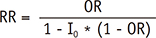 , where I0 is baseline risk of control group.2
, where I0 is baseline risk of control group.2
When the outcome is not rare, Poisson regression or log-binomial model are preferred to obtain RR instead of logistic regression.
Odds ratio as the measure of effects in case-control designs
When we are interested in a disease that is very rare, implementing a study with a cohort design is disadvantageous because not only it requires a long observation period and high cost but also it is very difficult to get sufficient information on occurrence of the disease. Case-control design offers a more efficient alternative in such a situation. In case-control design, subjects were selected from disease and no disease groups separately. The sample size of control group without disease is determined as appropriate, only considering the sample size of disease group. Therefore, there is no denominator which is needed to calculate a risk because information on the entire population is not collected. Computing both risk (p) and RR is impossible in the case-control design.
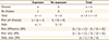
However, odds and OR, ratio of odds in exposed and unexposed group, can be easily obtained in this design. When the disease is very rare, we can use OR as an approximation of RR. Also different size of no disease group is applicable as the study design is needed. Table 3 shows the value of RR can be easily changed by only arbitrarily changing the size of no disease group from 1.91 to 1.98, while OR shows consistency having the same value of 2. Therefore, you should not use risk or RR inappropriately in studies with case-control design. When the outcome of interest has very low prevalence, OR calculated in case-control studies can be used as an approximation of RR.
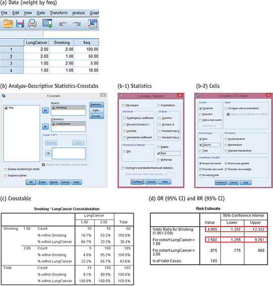
The procedure of obtaining OR and RR using IBM SPSS Statistics for Windows Version 23.0 (IBM Corp., Armonk, NY, USA)


 XML Download