

 PDF
PDF ePub
ePub Citation
 Print
Print


Introduction
Radiographic examination of the alveolar bone is an essential step in the diagnosis of dental diseases such as periodontitis, endodontic lesions, and dental ankylosis.123 In particular, assessments of the alveolar bone height, the thickness of cortical and cancellous bone, and the periodontal ligament space are key for diagnosing these diseases. The periodontal ligament space is an important indicator of the presence of a healthy and functional periodontal ligament, as well as the relationship between the tooth root and alveolar bone. Conventional intraoral radiography is adequate for determining the width of the interproximal periodontal ligament space and bony defects,45 but has some limitations in the depiction of buccolingual structures.6789
Recently, cone-beam computed tomography (CBCT) has been favored for periodontal evaluation because of its capability of 3-dimensional analysis.101112 Three-dimensional reconstruction of alveolar bone offers a precise diagnosis of furcation and intraosseous defects in order to plan periodontal surgery and regenerative therapy. CBCT also allows observation of the tooth root morphology; however, the root boundary is difficult to set definitively because CBCT images have no threshold to define the root dentin. Furthermore, image blurring can result from the partial volume effect and artifacts sometimes obscure the gray value of the boundary. To our knowledge, there have been no studies investigating the successful depiction of tooth root morphology in CBCT images. Clear discrimination of the periodontal ligament space could assist in visualizing the tooth root morphology.
The healthy periodontal ligament space is approximately 0.2 mm thick, and the spatial resolution of CBCT is sometimes insufficient to depict this space.131415 The spatial resolution of CBCT images is determined by many factors, including tube current, hardware specifications, and image reconstruction software. Although hardware specifications impose some fixed limitations,16 image reconstruction algorithms provide some flexibility. In recent years, research on several reconstruction algorithms of multi-slice computed tomography (CT) scans, such as iterative reconstruction, have been developed;17 however, the conventional filtered back-projection (FBP) method and the Feldkamp algorithm - one of the most widely referenced algorithms18 - are still popular approximations for dental CBCT reconstruction. Therefore, we have focused on the image reconstruction filter in the FBP algorithm to attempt to reduce image blur and improve spatial resolution.19 One key method to improve the results of CT imaging is changing the reconstruction filter to optimize image characteristics that depend on the region of interest. For example, in chest CT imaging, a reconstruction filter that emphasizes the high-frequency component has been applied,20 and in soft-tissue CT imaging, a reconstruction filter that suppresses the high-frequency component has been used. However, in dental CBCT applications, reconstruction filters are rarely available to alternate and improve image quality directly for diagnostic purposes, such as discerning a narrow space between structures with high CT values.
In this study, we examined various reconstruction filters in the FBP algorithm to evaluate the periodontal ligament space of a dry skull phantom as a sample of a narrow structure and to verify that the rendering of the fine, hard-tissue structures can be improved. We also evaluated the filters' physical and quantitative effects with the use of an experimental phantom.
Materials and Methods
Image acquisition and reconstruction
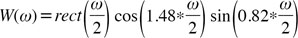
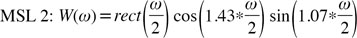
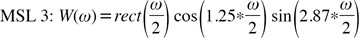
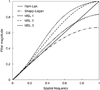
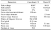
In this study, a dental CBCT scanner (Alphard-3030, Asahi Roentgen Industry Co. Ltd, Kyoto, Japan) was employed. Images were acquired from 4 different areas in 2 skull phantoms (Kyoto Kagaku Co. Ltd, Kyoto, Japan), a wire phantom, a water phantom, and an artificial periodontal ligament phantom. The CBCT exposure conditions are shown in Table 1. The CBCT scanner can acquire both raw projection data and reconstructed 2-dimensional axial images (the Alphard's default images). The default images from the Alphard device were reconstructed with its default application using a Shepp-Logan filter and additional confidential image processing. The raw projection data were reconstructed into modified axial images using 5 filters with a software package called Open Source Cone-beam Reconstructor (OSCaR).21 OSCaR is written in Matlab code (MathWorks Co. Ltd, Natick, MA, USA) and uses the FBP method and the Feldkamp algorithm. Two well-known filters (Ram-Lak and Shepp-Logan) were employed as references, and 3 filters were designed to increase the high-frequency component based on the Shepp-Logan function (Fig. 1).2223 The formulae of the filters were as follows:
Skull phantoms used for visual evaluations
CBCT data from 2 commercially available skull phantoms made with actual human dry skulls (age and sex unknown) embedded in soft tissue-equivalent resin were used for visual evaluation of periodontal ligament space visibility. The acquired image regions from the 2 skull phantoms included the maxillary anterior region and mandibular anterior region of 1 phantom and the mandibular anterior region and mandibular molar region of the other phantom.
The OSCaR reconstructed images and the default images of the skull phantoms were compared using the Thurstone method of paired comparison,24 and a scale value was calculated. Six image sets were compared using a round-robin formula for 4 different jaw regions. Image clarity of the periodontal ligament space boundaries was evaluated by 3 periodontists and 3 radiologists with >5 years of clinical experience. In total, 60 comparisons were performed by each observer. All observations were performed randomly on a 20.1-inch medical monitor (Radi-Force G20, EIZO Co. Ltd, Hakusan, Japan) operating at a resolution of 1200×1600 pixels. Before the viewing sessions, examiners were calibrated with test images and the evaluation point was explained. Examiners were allowed to change the window width/level and slice positions using ImageJ 1.47b software (a Java-based image processing program) and a Digital Imaging and Communications in Medicine viewer, both developed at the National Institutes of Health (MD, USA). Slice positions of the 2 observation images were synchronized, and an observational time limit was not specified. This observation study was approved by the Nagoya University ethics board (approval number 12-322).
The paired comparisons were statistically evaluated by analysis of variance using the F test (α<.05) and the yardstick method.25
Physical evaluation
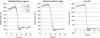
To confirm image characteristics, the modulation transfer function (MTF) and Wiener spectrum (WS) were calculated.26 The MTF, which is calculated from the point spread function, is the established method for characterizing the spatial response of an image. In this study, a wire method was employed for the MTF calculation,27 using a wire phantom made of copper wire (0.28 mm in diameter) and a water-filled cylindrical acrylic container (150 mm in diameter). The WS is a valuable tool for assessing the noise power of an image in the spatial frequency domain and was calculated by the virtual slit method,2829 using a cylindrical water phantom made only of a water-filled cylindrical acrylic container. Both calculations were performed using ImageJ visualization and measurement software and Excel 2010 (Microsoft Co., Ltd., Redmond, WA, USA). We assessed images using the default reconstruction of the Alphard apparatus and reconstruction with the filter that was rated highest for visual evaluation.
To distinguish the measurable periodontal ligament space widths as a parameter for periodontal ligament space visibility, we used the periodontal ligament phantom to compare the gray values between the alveolar bone equivalent and the simulated periodontal ligament space.
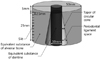
The periodontal ligament phantom was made from 2 different materials: an alveolar bone-equivalent substance and a dentin-equivalent substance produced as a solid column by Kyoto Kagaku Co. Ltd (Kyoto, Japan). The CT values of each block, confirmed by whole-body CT (Asteion Super 4 TSX-021B, Toshiba Medical Systems Co. Ltd, Otawara, Japan), were 272 and 1893, respectively. These blocks were shaped into a center post with a fixed circumference by Tokai Giken Co. Ltd (Ena, Japan) and then assembled to simulate a periodontal ligament space. The dimensional tolerance of the cutting work was estimated to be <0.02 mm. The composition of the materials and the final shape are shown in Figure 2. Tapering of a circular cone-shaped hole bored in the center of the circumference simulated changes in the width of the periodontal ligament space in the range of 0.0–1.0 mm. The periodontal ligament phantom was placed in water, and the periodontal ligament space filled with water to simulate biological conditions.
Axial images of the periodontal ligament phantom were obtained by CBCT (the default reconstruction and reconstruction with the highest rated filter) and microscopic CT (micro-CT high-resolution (R_mCT2, Rigaku Co. Ltd, Tokyo, Japan) as a reference. The microCT machine has microfocus X-ray tubes and a high-resolution flat-panel detector. The gantry is 194 mm in diameter, and the maximum field of view is 73×57 mm. The voxel size and the field of view were set to 0.1 mm3 and 48×48 mm, respectively. The phantom coordinate axes were adjusted to match those of the CBCT as much as possible. Exposure conditions using the microCT scanner are shown in Table 1. The acquired images of each modality were converted to gray values for each pixel, and the gray values of the periodontal ligament space and the alveolar bone were extracted using Excel 2010. To measure the periodontal ligament space, we compared the gray values of the periodontal ligament space and the alveolar bone in a total of 10 slices representing a 0.1-mm change in the periodontal ligament space. For the statistical treatment of the gray values, the lower threshold level showing the presence of bone was set at the lower limit of the 95% CI of alveolar bone. The 95% CI was approximately the same as the mean value±2 standard deviations (SDs). Thus, if the value obtained by subtracting the gray value of the estimated region of the periodontal ligament space from the mean value±2 SD of the alveolar bone was positive, it was considered to be a significant difference and confirmed the existence of a periodontal ligament space.
To visualize the effect of gray-value alteration by the reconstruction filter, the gray-value profiles of the periodontal ligament space were compared using polar-transformed images generated in ImageJ. The polar images were stacked at an angle to avoid any noise influence.
Results
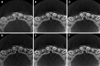
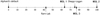
The representative images obtained from the skull phantoms are shown in Figure 3. The default images obtained using the Alphard apparatus were smooth, but the reconstructed images using the MSL function were rough in appearance. The raw choice matrix is shown in Table 2. The results of the Thurstone paired comparison using these images are shown in Figure 4. The resulting scale values were calculated as follows: default image: 0, Ram-Lak: 43, MSL 1: 64, Shepp-Logan: 76, MSL 3: 77, MSL 2: 100. The image that best distinguished the periodontal ligament space was the one reconstructed with MSL 2. The default images used in clinical settings yielded the worst result. The yardstick method revealed a significant difference between each filter, with differences in scale values ≥28. Thus, visibility of the periodontal ligament space was significantly poorer in the MSL 1, Ram-Lak, and Alphard default images than in the MSL 2 images.
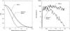
The MTF and WS values were compared, using water and wire phantoms, to verify the changes in image characteristics between MSL 2 and Alphard default images. The values for MTF and WS are shown in Figure 5. The MTF values reveal that the spatial resolution in the MSL 2 images was higher than that in the default images. The WS values increased when using a reconstruction filter that emphasized high-frequency components; MSL 2 images had particularly high WS values up to the high-frequency domain, which indicates greater granularity.
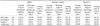
To confirm the minimum discriminable width, axial images of the periodontal ligament phantom reconstructed with 2 conditions were compared using the periodontal ligament phantom. The subtracted gray values of each condition are shown in Table 3. The gray cells represented the minimum values smaller than 2 SDs, and these cells were presumed to be the periodontal ligament space. A positive value indicated that the gray value of the periodontal ligament space was lower than the value of the mean -2 SDs of alveolar bone, and the periodontal ligament space was determined. A negative value indicated that the space could not be distinguished, because the periodontal ligament space was assimilated into the bone. Simulated periodontal ligament spaces thinner than 0.3 mm could not be observed under either condition. The discriminating width limits were 0.6 mm for the Alphard default images and 0.4 mm for the MSL 2 images.
The gray value profiles of the simulated periodontal ligament space are shown in Figure 6. The representative value of the simulated periodontal ligament space in the polar-transformed images is shown in Table 4. The MSL 2 profile represents a sharp decrease and a clear apex of gray values at the simulated space widths of 0.5 and 0.4 mm but not at the 0.3-mm profile. The Alphard default image profile showed a gentle degradation of gray values for each width. As a reference, the microCT profile demonstrated steady degradation of gray-value differences in relation to the reduction in size of the periodontal ligament space. The appearance of the profiles graphically explains the results of the statistical analysis with a 95% CI.
Discussion
In this study, the optimal reconstruction filter was MSL 2, which had a high-frequency component enhancement. The results of the paired comparisons revealed that the images enabled the observer to clearly view the boundary of the periodontal ligament space. The MTF and WS results confirmed that MSL 2 reconstruction improved image sharpness despite increased noise. These physical evaluations suggest that sharp images enhance the visualization of the periodontal ligament space; in other words, the visibility of the periodontal ligament space is not markedly affected by noise. Therefore, the images used for visual assessment by the observers were provided as a stack instead of a single slice. The observers recognized the continuous structure by comparing the plurality of slices and then provided a visual evaluation of the periodontal ligament space. The visual evaluation may have been less influenced by image noise in the setting of this study. The images for visualization of periodontal bone may use high-frequency enhancement. Therefore, our data comprise the essential components for precise visualization of periodontal hard-tissue structures.
The highest spatial resolution of the CBCT apparatus employed in this study was a square voxel of 0.1 mm. In the imaging mode with 0.1-mm3 resolution, the image reconstruction is performed using data mainly obtained from a decentralized area of the X-ray beam. However, we conducted the experiments in the imaging mode using the central area of the X-ray beam, although the spatial resolution was inferior. The spatial resolution could be considered insufficient for depicting the thickness of the periodontal ligament space; however, it is noteworthy that changing the reconstruction filter increased the spatial resolution under conditions that are generally applicable to many currently available devices.
This study successfully evaluated differences between images, even though the filtering effect was predicted to yield relatively small differences in CBCT images. Using the Thurstone paired-comparison method, which is effective in distinguishing similar subjects, we clearly distinguished differences between the reconstructed images and succeeded in scaling all the filters. The comparison of MSL 1 and MSL 2 shows that the enhancement of the high-frequency component had a maximum value, above which image degradation occurs. This degradation appears to be caused by 2 main factors: hard-tissue artifacts and noise enhancement by high-frequency enhancement. These results of the sensory and physical evaluations carried out in this study correspond well with the results of a previous study.19
In a quantitative assessment, the normal periodontal ligament width is difficult to depict with conventionally reconstructed CBCT images, partly because the space that exists between similar pixel values is difficult to visualize. 30 The default CBCT images resulted in the detection of a 0.4-0.6-mm interval; this was inferior to the results of a previous study.1415 This is partly because the periodontal ligament phantom replicated the nonuniform morphology of the periodontal ligament space, and the space was filled with water. Given the gradually changing width of the periodontal ligament space and the relatively large voxel size, it is likely that the partial volume effect influenced our results. Additionally, the periodontal ligament space was filled with water to mimic biological conditions; this was not the case in previous studies. Thus, our results, although inferior, may be closer to what may be achieved with living patients.
MSL 2 improves the resolution of dental CBCT without having to replace current hardware. This means that image quality can be improved with little associated expense or any increase in radiation dose - it only requires a software update. However, although sharp images were obtained by image processing, they were not sufficient to depict the periodontal ligament. To obtain sharper images, a high-resolution detector and an X-ray tube with a small focus are considered to be essential, but the exposure conditions eventually lead to an increase in the radiation dose.19 Because the right balance of noise and sharpness is required, a suitable reconstruction filter is useful in the dental field.
In conclusion, we determined that a high-frequency enhancement filter improved spatial resolution and allowed for better measurement of the periodontal ligament space. We also confirmed that using an image with a high-frequency component improved the evaluation of a periodontal ligament phantom. However, higher spatial resolution led to increased noise levels. This study was successful in finding a suitable reconstruction filter to discern the periodontal ligament space. However, for clinical applications, the various characteristics of image quality should be taken into account, including measurement of the contrast-to-noise ratio; this will require further optimization. Thus, future investigations can verify the clinical benefits of altering the reconstruction filter by ascertaining the importance of an appropriate compromise between sharpness and smoothing in order to achieve improved diagnostic accuracy or to save time. Apart from periodontal diagnosis, we believe that our method has the potential to improve periodontal treatment by using 3-dimensional visualization and stereolithography technology, especially in regenerative therapy when a scaffold material is applied. The development of clear and precise imaging techniques will improve such applications as part of periodontal treatment.


 XML Download