According to Korean law, drunk driving refers to driving with a blood alcohol concentration of 0.05 % or higher. Drunk driving is one of three major traffic violations together with hit-and-run and unlicensed driving. Although the overall incidence of traffic accidents has been decreasing steadily in Korea because of stricter regulations, and aggressive enforcement by police, the incidence of accidents resulting from drunk driving has not decreased.[1]

In 2012, a Korean local prosecutor's office requested the Department of Clinical Pharmacology and Therapeutics of Asan Medical Center, Ulsan University to estimate the blood alcohol concentration of a defendant during driving. The defendant was suspected of drunk driving. However, the suspect's blood alcohol concentration was measured after he had finished the driving using a breath alcohol test. The suspect stated that he had consumed four cups of soju at an average rate over a period of about 30 minutes just before driving. Blood alcohol concentration measured at 1 hour 24 minutes after the end of alcohol drinking over 30 minutes was 0.173%, as estimated by the alcohol breath test.

In this study, modeling and simulation analysis estimated the possible alcohol concentration in blood over time while the defendant was driving using a Bayesian method based on the alcohol consumption history reported by the defendant, blood alcohol concentration measured by the alcohol breath test, and a population pharmacokinetic (PK) model of alcohol, previously developed for Korean adult males. This approach provided scientific evidence of the defendant's blood alcohol concentration during a specific time window, which could be useful during prosecutions for drunk driving.

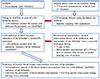
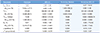
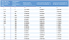
An alcohol PK model (Original, Alcohol PK Model, OAPKM), previously developed using 178 blood alcohol concentrations (%) measured by the breath alcohol test from 24 healthy, Korean adult males in a phase 1 clinical trial (Table 1), was used in this analysis. OAPKM is one compartment model with linear absorption, and saturable elimination, consisting of absorption rate constant (K_a), central volume of distribution (V_d) and Michaelis- Menten equation for the elimination.[2] In the OAPKM, body weight is associated with both V_d and the maximum elimination rate (V_max) in the Michaelis-Menten equation. Using this OAPKM and the alcohol drinking history, and the measured blood alcohol concentration of the defendant, Maximum a posteriori (MAP) Bayesian prediction was conducted to estimate blood alcohol concentrations over time.[23] The defendant was assumed to have consumed a total of 32 mg (4 cups × 8 mg/cup) of alcohol based on the usual alcohol concentration in soju (20%) and the volume of a small cup for soju (40 ml). To ensure generalizability and to reflect parameter uncertainty, a non-parametric bootstrap analysis was applied to the Bayesian prediction.[456] Specifically, 1,000 different datasets were generated by random sampling with replacement from the original PK data used to build OAPKM. Repetitive model fittings were then performed 1,000 times using the OAPKM and each of 1,000 bootstrap datasets. Using the resultant 1,000 different population PK parameters estimated from this bootstrap (BAPPKP, Alcohol Population PK Parameters estimated from Bootstrap), and the alcohol consumption history (amount, time), blood alcohol concentration, and body weight of the defendant, 1,000 replicates of the MAP Bayesian estimation of the individual alcohol PK parameters of the defendant (MAPIPKP, Individual PK Parameter estimated from MAP Bayesian Method) were performed using MAXEVAL=0 in NONMEM (version 7.2). Then, the possible blood alcohol concentrations over time were predicted, using the 1,000 MAP estimates, and the probability that the blood alcohol concentrations of the defendant during driving were 0.05% or higher was calculated (Fig. 1). To simplify the process, $SUPERPROBLEM in NONMEM was used, and repetitive batch processing including bootstrap data generation, NONMEM fitting, and Bayesian estimation were performed using R (version 3.01).

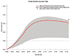
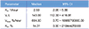
The bootstrap result of the original alcohol PK model from 24 healthy, Korean male, subjects was similar to the original PK parameter estimates of the single run in terms of median and the 95% confidence interval, suggesting that the resultant individual PK parameter estimates were reasonable (Table 1). The MAP estimates of the alcohol PK parameters of the defendant (MAPIPKP) were different from the PK parameters of the OAPKM. V_max and alcohol concentration at half of V_max (K_m) in the Michaelis-Menten equation constituting the OAPKM were considerably larger, while K_a and V_d were smaller than those in the OAPKM (Table 2). The MAPIPKP was used to create a blood alcohol concentration profile over time, and the result is shown with median and the 95% prediction interval (Fig. 2). The results showed a high probability that the blood alcohol concentration of the defendant was ≥ 0.05 % during driving (Table 3).

In the present analysis, the blood alcohol concentration profile of a defendant suspected of drunk driving was estimated using a previous alcohol PK model and the defendant's-specific information.

In some replicates of this bootstrap-Bayesian estimation analysis, estimation by NONMEM was terminated or individual Bayesian PK parameter estimates of the defendant (MAPIPKP) were unrealistic. We included all these terminated and unrealistic bootstrap results in the analysis. The minimization termination status of NONMEM has been reported to affect minimally the bootstrap result in previous studies.[78] Concerning the unrealistic PK parameter values of the defendant obtained during this analysis, we suggest that they were due to the inaccuracy of the defendant's statement about his alcohol consumption, rather than to a problem in parameter estimation.

MAPIPKP differed from those of healthy normal volunteers (parameters in OAPKM), and the blood alcohol concentrations of the defendant measured by the breath alcohol test were higher than the upper limit of the 95% prediction interval for blood alcohol concentration (Fig. 2). Specifically, the K_m in the MAPIPKP was approximately 30-fold higher than that in OAPKM (14.31% vs. 0.47%), whereas the V_max was only 9-fold higher (compared to 30-fold higher K_m) in the MAPIPKP (604.30%/ hour vs. 72.40%/hour). These results indicate that the alcohol elimination rate (^V_max/_(km+Ca), where C_A is alcohol concentration) of the defendant was much lower than that of an average healthy, Korean, adult male, which would be rare. One possible explanation is that the amount of alcohol consumption stated by the defendant was lower than the actual one. The defendant could have under-reported the amount of alcohol he consumed, in which case the PK parameters estimated by the Bayesian methods would be biased.

The current Bayesian approach to estimate blood alcohol concentrations during driving provides a good example of the application of PK modeling and simulation to an area other than patient treatment or drug development. The estimated alcohol concentrations provide scientific evidence that could be useful in a trial. The present analysis could represent a starting point for the application of quantitative clinical pharmacology principles to social areas outside medicine.