The time course of drug action combines the principles of pharmacokinetics and pharmacodynamics. Pharmacokinetics describes the time course of concentration while pharmacodynamics describes how effects change with concentration. There are 3 ways to think of the time course of effects:

This tutorial outlines the basic principles of the concentration-effect relationship (pharmacodynamics) and illustrates the application of pharmacokinetics and pharmacodynamics to predict the time course of immediate drug effects.

Drug concentration is not as easily observable as doses and effects. It is believed to be the linking factor that explains the time course of effects after a drug dose.

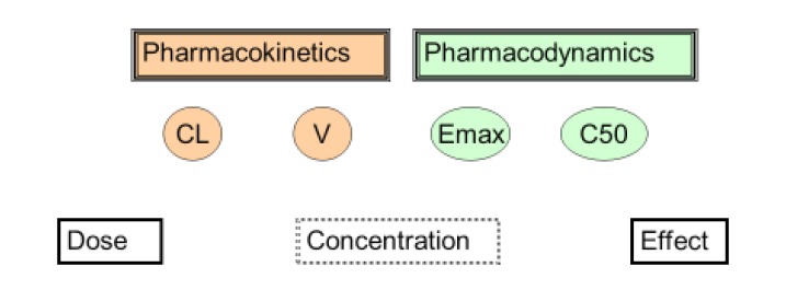
The science linking dose and concentration is pharmacokinetics. The two main pharmacokinetic properties of a drug are clearance (CL) and volume of distribution (V).

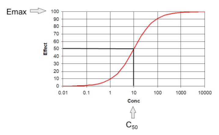
The science linking concentration and effect is pharmacodynamics. The two main pharmacodynamic properties of a drug are the maximum effect (Emax) and the concentration producing 50% of the maximum effect (C₅₀). The C₅₀ is also known as EC₅₀ but C₅₀ is preferred to make it clearer this is a concentration and not an effect scaled parameter.

Clinical pharmacology describes the effects of drugs in humans. One way to think about the scope of clinical pharmacology is to understand the factors linking dose to effect. Clinical pharmacology may be defined as the science of understanding how to achieve a desired clinical effect by administering the right dose. This can be done by choosing a target effect, using pharmacodynamics to predict the target concentration which produces the effect and then using pharmacokinetics to predict the dose (Fig. 1).

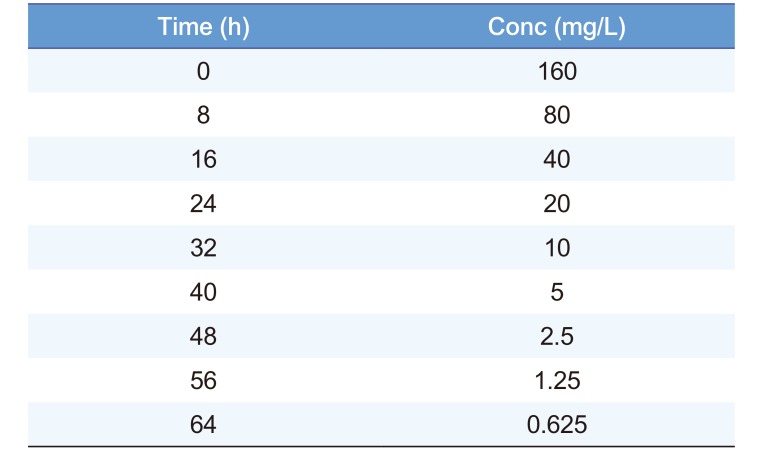
The time course of drug concentration can be described in terms of half-life. Table 1 shows an example of times and concentrations which can be used to find the half-life. The half-life is 8 h because the concentration falls by 50% during each 8 h time interval.

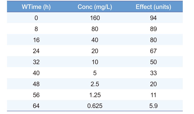
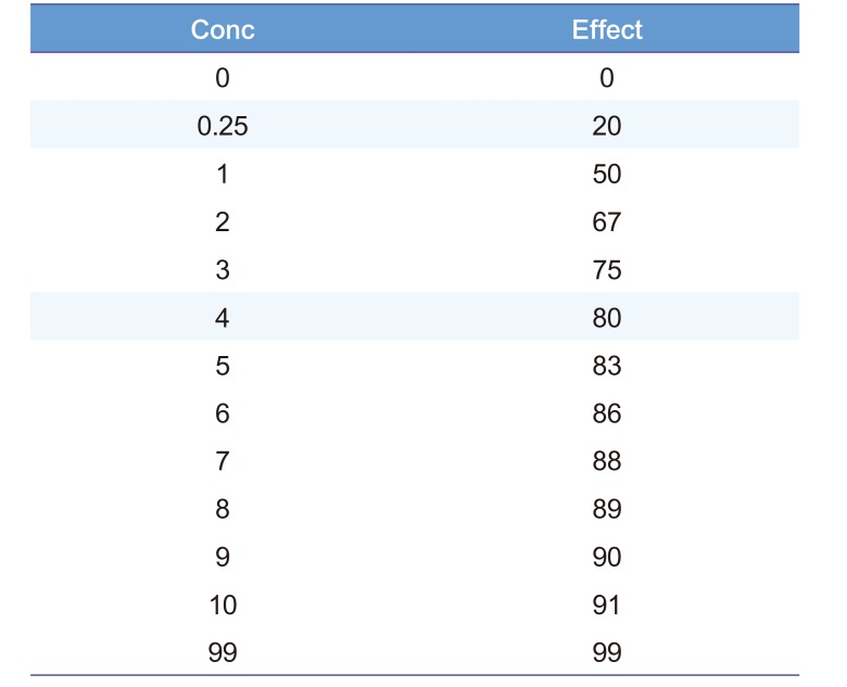
The time course of drug effect can be described using the C₅₀. Table 2 shows an example of times and effects which can be used to find the C₅₀ but this also requires a guess of the value of Emax. Emax is a parameter which cannot be directly observed because an effect equal to Emax only occurs when concentration is infinite. Infinite concentrations cannot be achieved in any real life circumstance. The time course of effect can be used to estimate (a sophisticated word for guess) the Emax. Looking at Table 2 the highest effect is 94 units. If we guess that Emax is 100 then by definition the concentration producing an effect of 50 is the C₅₀. This C₅₀ concentration is 10 mg/L.

The relationship between concentration and effect in Table 2 is plotted in Figure 2. It can be seen that above C₅₀ the effect increases more and more slowly as concentration increases. This is an important property of the Emax model that is the basis of pharmacodynamics. Based on the law of mass action, the binding of a drug to a receptor should follow a hyperbolic curve (as shown in Fig. 2). If it is assumed that the effect is directly proportional to the binding then the C₅₀ will be the same as the Kd. The Kd is the equilibrium binding constant. It is the concentration of unbound drug at which 50% of binding sites are occupied. Notice that Emax can never be directly observed. It is the asymptotic effect of the drug at infinite concentration. Even 10 times the C₅₀ only reaches 90% of Emax.

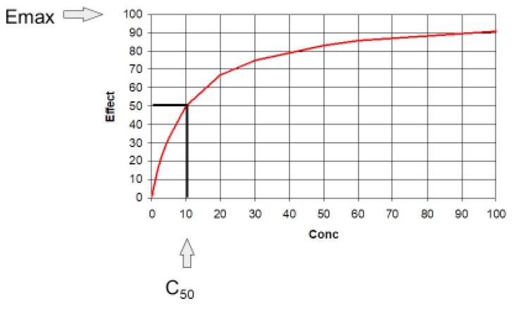
Figure 3 shows the identical values for concentration and effect as that shown on the previous figure. The only change is in the X-axis of the graph to a logarithmic scale.

The log transformation changes the shape of the curve so that it now looks “S-shaped” (sigmoid) but this is not a sign of a sigmoid Emax model (see later). The transformed X-axis allows a wider range of concentrations to be plotted and it can be seen that at very high concentrations the effect approaches Emax.

The portion of the curve between 20 and 80% of Emax is approximately a straight line. This almost linear relationship was helpful before the days of computers because the slope could be described by simple calculations.

Older textbooks commonly refer to ‘log-dose response curves’. It is important to appreciate that there is no underlying biological or physical reason to think that drug effects are related more closely to the log of concentration than untransformed concentrations.

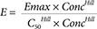
A problem arises from thinking that effects are related to the log of concentration when the concentration is known to be zero (Equation 1):

At zero concentration is obvious that the effect must be zero but the log of zero is mathematically undefined and so the effect is also undefined. The log concentration model also does not recognize that effects will approach a maximum which is always the case for biological systems.

The log transformation is useful for visualising a wide range of concentrations but the log concentration model has no basis in pharmacological theory.

The Emax model (Equation 2) is the most fundamental description of the concentration effect relationship. It has strong theoretical support from the physicochemical principles governing binding of drug to a receptor (the law of mass action). All biological responses must reach a maximum and this is an important prediction of the Emax model.

When concentrations are low in relation to the C₅₀ then the concentration effect relationship can be approximated by a straight line (the linear pharmacodynamic model, Equation 3):

Table 3 shows some useful predicted effect values in relation to concentrations expressed as multiples of the C₅₀. There are two other useful concentrations to remember: C₂₀ - the concentration at 20% of Emax. It is ¼ of C₅₀ and C₈₀ - the concentration at 80% of Emax. It is 4 times the C₅₀. This means the Emax model predicts a 16 times change in concentration is needed to change the effect from 20 to 80% of Emax. Note that doubling the concentration from C₅₀ to 2 times the C₅₀ only increases the effect by 17%.

Many drugs seem to have a steeper relationship of concentration and effect so that a smaller change is required to increase the effect from 20% to 80% of Emax. These steeper relationships can be described by the sigmoid Emax model.

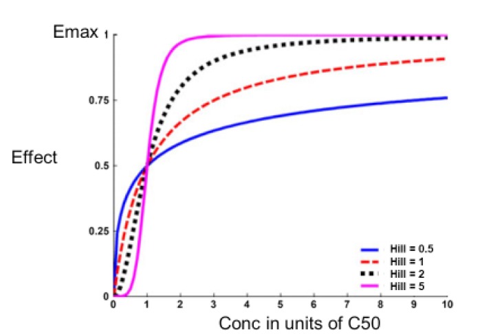
In 1910, the physiologist Hill was investigating the shape of the oxygen - haemoglobin saturation relationship.[1] He noted it was steeper than the simple binding predictions of the Emax model. By trial and error he found that by adding an exponential parameter to the concentration and C₅₀ terms in the model the shape of the relationship could be made steeper. This extra parameter is known as the Hill exponent (Equation 4).

Subsequently the molecular biologist Perutz won a Nobel prize for describing the structure of haemoglobin which incorporates 4 binding sites for oxygen.[2] The binding of each oxygen atom affects the other binding sites and causes the steep oxygen-haemoglobin binding curve.

The application of the sigmoid Emax model in pharmacology has been reviewed by Goutelle and colleagues.[3] Examples of the shape of the sigmoid Emax model compared with the Emax model (Hill=1) are shown in Figure 4.

Theophylline is used to treat severe asthma. It is a bronchodilator. Airway constriction slows the peak flow rate of air from the lungs. Theophylline can increase the peak flow rate and as an C₅₀ of about 10 mg/L. The maximum effect of theophylline (Emax) is to increase peak flow by 100% above the baseline peak flow. Three scenarios are shown here to illustrate the time course of effect with different initial concentrations using the theophylline pharmacodynamic parameters.

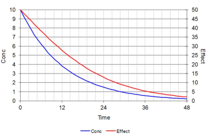
Figure 5 is the first of three figures showing how the time course of immediate drug effect depends upon the initial concentration as well as the pharmacokinetics of the drug.

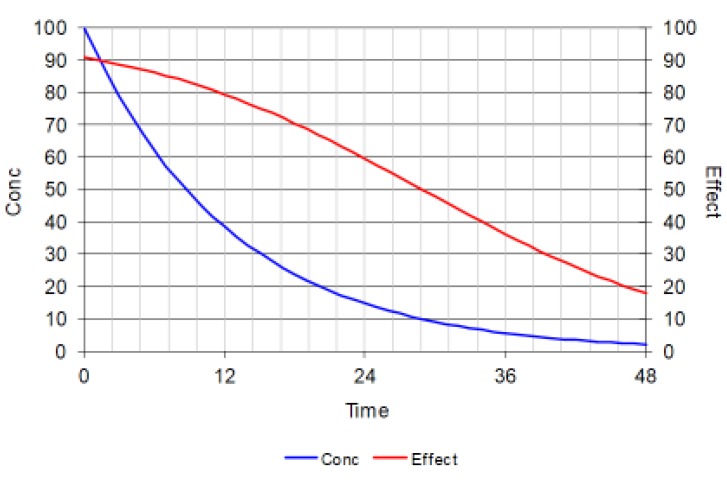
Each figure shows the time course of concentration (blue line) after a bolus dose at time zero. The half-life is about 9 hours (similar to theophylline). The initial concentration is 10 times the C₅₀ for theophylline and this produces an initial effect of 90% of Emax (red line).

Figure 5 shows that after one half-life the concentration is halved but the effect has changed by less than 10%. As concentration falls the effect disappears more quickly.

If a smaller dose is given so that the initial concentration is the same as the C₅₀ then the initial effect will only be 50% of Emax. At these lower concentrations the time course of effect is almost parallel to the time course of concentration.

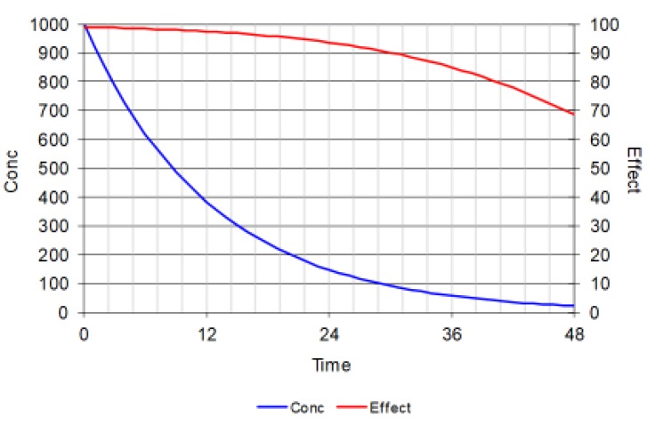
When a very big dose is given so that the initial concentration is 100 times the C₅₀ then the initial effect is close to 100% of Emax. The effect changes very little despite big changes in drug concentration. After more than 5 half-lives when nearly all the initial dose will have been eliminated from the body the effect is still 70% of Emax.

his figure is important because it shows how drugs which have short half-lives can have big effects even if the dosing interval is many half-lives. This is quite common for receptor antagonists e.g. beta-blockers and angiotensin-converting enzyme inhibitors.

In summary the time course of effect can be described by three regions by considering if concentrations are above the C₈₀ or below the C₂₀ (Fig. 8).

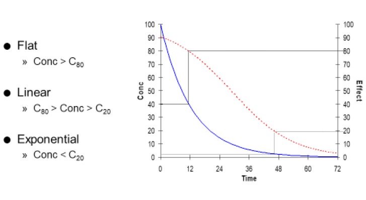
When concentrations are very high (greater than C₈₀) the curve is almost flat. There is little change in effect despite big changes in concentration.

When concentrations are very low (less than C₂₀) the curve is almost exponential. The time course of concentration and effect are almost parallel to one another. This is the only time it makes sense to describe the effect as having a ‘half-life’.

In between the C₂₀ and C₈₀ the time course of loss of drug effect is almost a straight line.

Figure 9 looks like a complicated figure but it illustrates a very simple principle -- “If the dose of a drug is doubled then the duration of response will increase by one half-life.”

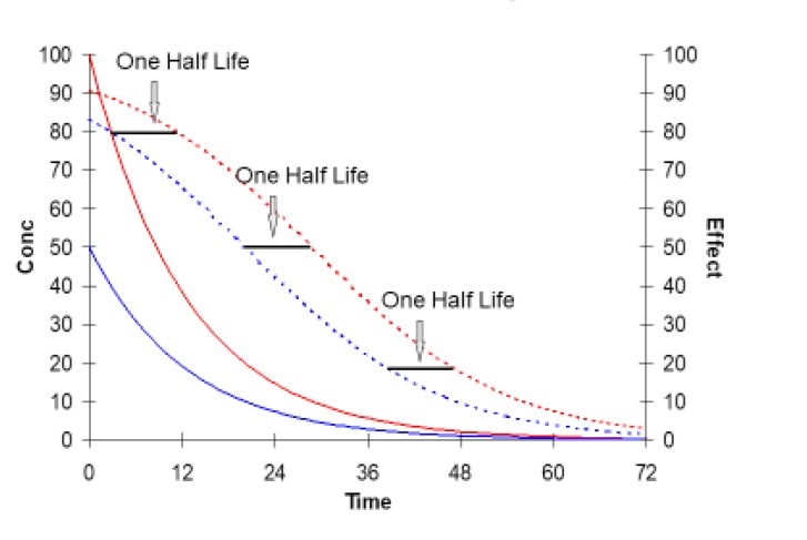
The duration of response means the time that the drug effect is above a pre-defined critical value e.g. the time above 50% of Emax. With a low dose (blue lines) the duration of effect is about 20 hours. At 20 h the concentration is equal to 10 mg/L (the C₅₀).

Doubling the dose (red lines) prolongs the duration of effect to nearly 30 h (duration increased by one half life). At 30 h the concentration is equal once again to 10 mg/L - with the same level of effect (50) that was used to mark the end of the response for the lower dose.

The increase in duration of response from doubling the dose is independent of the size of effect that is chosen to mark the end of the response.

Go to :

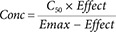
One of the most important applications of the Emax model is to translate the desired clinical effect (the target effect) into a target concentration (Equation 5).

Re-arrangement of the Emax equation leads to a prediction of the target concentration to reach the target effect.

Selection of a dosing interval so sustain a desired level of effect has to take into account the time course of effect. In the simplest case this depends on both the half-life and the C₅₀.

Many drugs (e.g. beta-blockers, ACE inhibitors and prednisone/prednisolone) have half lives of a few hours but are effective with once daily dosing. This can be explained by concentrations being above the C₅₀ for most of the day.

Concentration effect curves are non-linear (Emax model) effects do not increase in direct proportion to the dose. This leads to these 2 key insights about pharmacodynamics and the time course of drug effect:

Go to :