Quantification of Gadolinium Concentration Using GRE and UTE Sequences

So Hee Park; Yoonho Nam; Hyun Seok Choi; Seung Tae Woo

doi:10.13104/imri.2017.21.3.171

Abstract

Purpose

To compare different MR sequences for quantification of gadolinium concentration.

Materials and Methods

Gadolinium contrast agents were diluted into 36 different concentrations. They were scanned using gradient echo (GRE) and ultrashort echo time (UTE) and R1, R2* and phase values were estimated from collected data. For analysis, ROI masks were made for each concentration and then ROI value was measured by mean and standard deviation from the estimated quantitative maps. Correlation analysis was performed and correlation coefficient was calculated.

Results

Using GRE sequence, R1 showed a strong linear correlation at concentrations of 10 mM or less, and R2* showed a strong linear correlation between 10 to 100 mM. The phase of GRE generally exhibited a negative linear relationship for concentrations of 100 mM or less. In the case of UTE, the phase had a strong negative linear relationship at concentrations 100 mM or above.

Conclusion

R1, which was calculated by conventional GRE, showed a high performance of quantification for lower concentrations, with a correlation coefficient of 0.966 (10 mM or less). R2* showed stronger potential for higher concentrations with a correlation coefficient of 0.984 (10 to 100 mM), and UTE phase showed potential for even higher concentrations with a correlation coefficient of 0.992 (100 mM or above).

INTRODUCTION

The gadolinium contrast is the most representative paramagnetic contrast agent which is frequently used in clinical practice and research. Magnetic resonance imaging (MRI) using gadolinium contrast has enhanced the accuracy of diagnosis of Infection, inflammation, tumor and related vascular diseases (1). Gadolinium is known as a safe contrast media, however it may cause nephrogenic system fibrosis for those who have impaired renal function. Therefore, the careful use of gadolinium is recommended (2). It has been reported that deposition of injected gadolinium contrast agent was found at the basal ganglia and the dentate nucleus of the brain from patients who have not had kidney dysfunction (3). Therefore, the issue regarding how to use gadolinium effectively has become a prominent topic.

If quantitative measurement of gadolinium contrast agent is feasible, it will be possible to optimize the MRI protocol to maximize the diagnostic effect with minimum usage of contrast agent (4). Previous quantitative measurements of gadolinium in vivo were collected by measuring R1 relaxation time (5). However, the method using R1 relaxation time is not always accurate because it shows a nonlinear relationship in range of high gadolinium concentration. Moreover, since a correction of B1 inhomogeneity is necessary in order to collect the accurate R1 relaxation time, issues may arise, such as causing a delay in gathering MR images. Recently, research regarding quantification of gadolinium using phase information of gradient echo sequences (GRE) and quantification of high concentration using ultrashort echo time (UTE) are reported (6 7). However, those studies were conducted using a limited range of gadolinium concentration. Therefore, there is not much research conducted using different kinds of quantitative methods with a wider range of gadolinium concentration.

In this research, we compared different MR sequences in a wide range of gadolinium contrast agent concentrations via phantom study (8). We used two methods: multi-echo GRE using variable flip angle to measure R1, R2* and phase, and UTE to measure R1 and phase.

MATERIALS AND METHODS

Data Acquisition

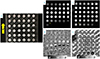
All MR experiments were performed on a 3T clinical scanner (Verio, Siemens, Erlangen, Germany) with a 12-channel phased-array head coil. A gadolinium contrast agent (Gadovist, Schering, Berlin, Germany) was diluted into 36 different concentrations as illustrated in Figure 1a (0.0125 to 1000 mM). The diluted contrast agents were filled into plastic vials and embedded into a plastic-filled container which has multiple crafted holes for vial insertion. The container was placed in a direction such that vials were perpendicular to the main magnetic field direction. The phantom was scanned using two different imaging sequences (GRE and UTE). To estimate the R1 values, multiple scans with different flip angles were performed for both sequences. To estimate R2* values, multiple echoes were obtained for GRE imaging. Imaging acquisition parameters for GRE included: TR = 7.5 ms, TE = 1.85/3.26/4.76 ms, flip angle = 3/6/9/12/15°, bandwidth = 1002 Hz/pixel, 1.0 mm isotropic voxel size. Imaging acquisition parameters for UTE included: TR = 7.5 ms, TE = 0.1 ms, flip angle = 3/6/9°, bandwidth = 650 Hz/pixel, 1.0 mm isotropic voxel size.

Image Processing

From collected MR data, R1 and phase maps from GRE and UTE were calculated. Also, a R2* map was calculated from multi-echo GRE data.

R1 estimation

MR signal for different flip angles can be represented by the following equation.

[Eq. 1]

s (θ) = M_{0} s i n θ \frac{1 - E_{1}}{1 - E_{1} c o s θ}

where E₁ = exp(-TR R1), M₀ and 0 represent proton density and flip angle, respectively.

R1 value was estimated using a nonlinear least-square curve fitting algorithm.

Phase estimation

Collected MRI Phase not only contains information about the gadolinium phase, but also contains global phase values from different causes. Because the global phase has relatively smaller spatial variation than the phase caused by gadolinium, global phase was estimated from the unwrapped phase images by 6th order polynomial fitting, then subtracted. In this step, the phase was unwrapped using a Laplacian unwrapping algorithm (9). Then, phases were divided by echo time for normalization. In case of using GRE method, phase value was collected from 1st echo image because high concentration of the tube showed very low SNR at another echo images.

R2* estimation

R2* was estimated from multi-echo data using the following equation.

[Eq. 2]

S(TE) = M₀exp(-TE R₂*)

R2* value was estimated using a nonlinear least-square curve fitting algorithm. All post-processing were performed in MATLAB 2016b (Mathworks Inc., Natick, MA, USA).

Image Analysis

To investigate the performance of gadolinium quantification, an ROI mask was made for each tube region from a magnitude image, then mean and standard deviation for each tube's concentration was calculated from estimated quantitative maps (R1, R2* phase). Concentration of gadolinium was divided into three sections (0 mM to 1 mM, 1 mM to 10 mM, and 10 mM to 100 mM) then Pearson correlation coefficient was calculated at each section.

RESULTS

Magnitude Images

UTE magnitude shows similar trend with GRE magnitude, but UTE magnitude detected a signal up to 500 mM, while GRE magnitude showed valid signal only up to 100 mM. Signal intensity of GRE magnitude had a slight increase from the start to 6 mM, then the intensity reached a flat line. Signal intensity of UTE magnitude was similar with that of GRE, which continued in a flat line until concentration reached 100 mM. UTE phase decreased from concentration 100 mM to 500 mM and showed a strong negative linear relationship (Fig. 1).

GRE Analysis

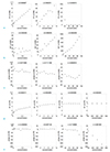
GRE data collected from concentrations of 100 mM or above were excluded since detected signal was similar to noise level. In the case of GRE magnitude, signal intensity of R1 tends to increase until approximately 6 mM, but the intensity tends to decrease at higher concentrations. R1 of GRE showed a strong linear correlation at concentration 10 mM or less with a correlation coefficient of 0.966 approximate. Specifically, the highest correlation value was measured from concentrations 1 mM or less with a correlation coefficient of 0.999 (Fig. 2a).

Signal intensity of R2* kept the increasing tendency from the starting concentration, but the intensity was unstable until the concentration reached 6 mM. Signal showed stability from concentration 10 mM. R2* of GRE showed a strong linear correlation at concentrations between 10 to 100 mM with a correlation coefficient of 0.984 (Fig. 2b).

Signal intensity from GRE phase showed that signal continuously but unstably decreased from the start. Signal generally had a negative linear relationship for concentrations 100 mM or less, but the correlation coefficient was lower than that measured from R1 and R2* of GRE (0.672,0.711, and 0.604 in respective ranges of concentrations) (Fig. 2c).

UTE Analysis

In case of UTE, both R1 and phase showed low correlation coefficient values at concentrations 100 mM or less compared to GRE, but phase data showed a strong negative linear relationship at concentrations 100 mM or above with a correlation coefficient of 0.992 (Fig. 2d, e).

DISCUSSION

In this research, we tested the potential for parameter quantification of R1, R2* and phase at various concentration ranges of gadolinium contrast agent. As shown in the previous studies, with respect to the contrast agent concentrations of 10 mM or less, R1, which was calculated by conventional GRE, showed a high potential for optimizing quantification. However, for higher concentrations, R2* showed a higher potential, and UTE phase showed potential for much higher concentrations. In practice, it is rare to use gadolinium contrast agent concentrations that are 100 mM or above in vivo, but in the case of superparamagnetic iron oxide application, there may be occasions where it would be difficult to optimize quantification, by applying the conventional method due to high magnetization, locally (10). Therefore, we expect that UTE phase could overcome the limit of using conventional methods for those applications.

The current study has a few limitations. First, the study was only performed in a phantom environment. Since there are several factors that interfere with quantification in vivo, they shall be taken into account. Second, in order to conduct an accurate R1 mapping, it is necessary to consider B1 inhomogeneity and obtain higher flip angle data than the variable flip angle method (11). In our study, the highest flip angle could only be used up to 9°, due to the limitation of UTE sequence. This can be a factor in decreasing the accuracy of R1 measurement through UTE; and the actual result also shows a discrepancy with the R1 value measured by GRE method at low contrast agent concentration. Lastly, in order to eliminate the background phase signals accurately in phase processing, a reliable phase signal is needed at the outside of the tube. However, the phase signals are not obtained because the gap between the tubes is filled with plastic material.