

 PDF
PDF ePub
ePub Citation
 Print
Print


The knee joint is basically a hinge joint with the main movement of flexion-extension. However, the radius and the length of the articular surface of the femur and tibia differ at the knee joint.12) As a result, a complex movement, which includes "sliding", actually occurs at a certain interval, in addition to rolling between the two bones.1) This allows the knee joint to move smoothly. At terminal extension, the knee joint is slightly hyperextended and stabilized with the tightening of the cruciate and collateral ligaments. As the length of the medial femoral condyle is longer than the length of the lateral condyle, the tibia rotates externally about 15° on the femur during the last 20° of extension. This kinematic phenomenon is well known, and it is called the screw-home movement.12345) Researches on the unique kinematics of the knee joint will provide essential data for the study and treatment of various knee diseases such as sports injury, artificial joint replacement, and others.1456789)
Various kinematic studies on knee joint movements have been conducted in an artificial or biological environment. Ishii et al.3) analyzed the flexion-extension movement by inserting pins directly into the femur and tibia. Some researchers used single plane or biplane radiographs, 3-dimensional (3D) magnetic resonance imaging, or computed tomography (CT) images for the study.45610) However, most of these studies analyzed a series of images at different knee flexion angles taken under static conditions, which might not reflect the dynamic knee motion that occurs during actual gait. Even though the methods using single plane or biplane radiographs or CT images were dynamic studies of in vivo knee kinematics, this can lead to unnecessary exposure to radiation.11121314) Gait analysis, using the 3D motion capture technique, is another research technique that enables the estimation of dynamic joint kinematics while walking on a straight footpath or running on a treadmill and radiation exposure is not necessary. However, data might be influenced by the attachment of skin markers. The skin is quite pliable, and hence, care needs to be taken during placement of skin markers to minimize the errors. Little has been reported on kinematics of the knee joint using 3D motion capture analysis during gait.
The purpose of this study was to analyze gender-based differences in healthy knee kinematics, especially the degree of rotational movement, during gait using the 3D motion capture technique consisting of an optical tracking system and associated software. The secondary purpose of this study was to compare dynamic knee joint kinematics between the dominant and non-dominant lower limbs during gait. We hypothesized that there would be no difference in dynamic knee joint kinematics between genders, and between dominant and non-dominant lower limbs during gait.
METHODS
This study was performed according to the protocol approved by the Institutional Review Board at Eulji University Hospital. All subjects provided informed consent to participate in this study. This study was conducted in volunteers with normal gait who had no history of musculoskeletal disease and injury or pain in the lower limbs, and no abnormalities on the anteroposterior hip-to-ankle radiographs with the patient standing and physical examinations. The study group was selected from among medical students who had volunteered to participate in this study. A total of 30 students, 15 males and 15 females, participated in this study. The mean ages were 20.3 years for males and 20.5 years for females. Subjects' height, weight, foot length, foot width, ankle width, knee width, and lower limb length were measured for the preliminary data of gait analysis. Deformities of the lower limbs were checked on the scanogram of lower extremities. To check for the torsional abnormalities, degrees of rotational profiles and anteversion by palpation of the greater trochanter in the prone position were measured. Foot deformities were also checked by the examiner.
The 3D motion capture of dynamic knee kinematics was estimated using an optical tracking system (Motion Analysis Co., Santa Rosa, CA, USA), which required at least three non-collinear markers on each bone. This system was composed of six synchronized infrared cameras placed circumferentially around the subject being examined. The frequency of motion capture was set at 120 Hz and the walking length for motion capture was set at 7 m.
We used three software programs for data processing; Eva Real Time (EvaRT ver. 4.2, Motion Analysis Co.), Orthotrak (Motion Analysis Co.), and Skeletal Builder (SKB, Motion Analysis Co.). EvaRT is the basic capture software for processing the data obtained from cameras. Orthotrak converts the database from EvaRT to 3D graphics automatically. SKB enables the calculation of the motion captured data from EvaRT. Two virtual planes were formed using the SKB program in this study, and the relative movement between these two virtual planes was calculated.
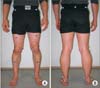
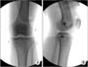
Then, 9-mm passive reflective markers (Motion Analysis Co.) were attached by using the Helen-Hayes method,15) and additional markers were attached to the medial and lateral condyles of the proximal tibia, on which the medial and lateral collateral ligaments are attached (Fig. 1). To minimize the error while positioning the four markers on the medial and lateral condyles of the femur and tibia, the marker position was checked using C-arm fluoroscopy during the early stage of the study in all cases by an orthopaedic resident. The marker on the lateral tibial condyle was positioned just over the top of the fibular head, while the marker on the medial tibial condyle was positioned over the bony surface on which the medial collateral ligament is inserted. It was mostly at the same level as that of the lateral tibial condyle marker (Fig. 2).
To capture the data, the subjects were asked to stand in the center of the capture volume, and the markers were attached. The static data was captured while the subjects stood at the center of walking volume. To capture the dynamic data, the subjects were directed to walk along the walkway (7 m) for more than five times. The mean value was obtained by gathering the data three times. For assessing gait velocity, the subjects were instructed to walk at a constant pace of 90 steps per minute. Before dynamic data were obtained, the subjects were given several practice trials to ensure that they understood the proper walking technique and timing. The temporal parameters of gait were measured using the Orthotrak program, and kinematic data was obtained in 3Ds of the sagittal plane, coronal plane, and transverse plane. The data of each subject was displayed on an excel spreadsheet by dividing the gait cycle into 100-time periods (%). The data was also displayed in several graphs using the Orthotrak program to confirm whether the kinematics and kinetics of the subjects were similar to the gait of normal adults.
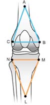
For this study, two virtual planes (the femoral coronal plane [Pf] and tibial coronal plane [Pt]) were created using the SKB program (Fig. 3). The lower leg marker was attached on the front side of proximal one-third of the lower leg. The line connecting the two proximal markers (M and N in Fig. 3) almost matched the flexion-extension axis of the proximal tibial articular surface. The relative movement of the virtual Pt, as to the virtual Pf, was measured by the degree of freedom in 3Ds. The coordinate system was defined as follows: the valgus/varus angle (+/-) was measured on the coronal plane (x-axis), while the internal rotation/external rotation angle (+/-) was measured on the transverse plane (y-axis). The flexion/extension angle (+/-) was measured on the sagittal plane (z-axis).
Statistical Analysis
The Wilcoxon paired t-test was used to analyze demographic data, gender-based difference in healthy knee kinematics, and dynamic knee joint kinematics between the dominant and non-dominant lower limbs during gait. All statistical analyses were performed using PASW ver. 18. (SPSS Inc., Chicago, IL, USA). A p-value less than 0.05 was considered statistically significant.
RESULTS
Physical Examination, Gait Linear Index, and Kinematics
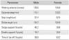
The mean heights were 174 cm (range, 165 to 185 cm) in males and 161 cm (range, 156 to 168 cm) in females, respectively. The mean weights were 71 kg (range, 59 to 80 kg) and 52 kg (range, 42 to 61 kg) in males and females, respectively. The mean age of males and females was 20 years (range, 18 to 25 years) and 20 years (range, 18 to 24 years), respectively. All subjects were right-lower limb dominant. With respect to the linear parameters of gait and kinematic data, there was no statistically significant difference between the male and female groups (Table 1).
Relative Movement of Virtual Tibial Coronal Plane for the Virtual Femoral Coronal Plane
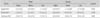
The mean changes in the rotational movement in three planes (sagittal, coronal, and transverse planes) between both knees and the mean changes in the knee angle in three planes between genders are summarized in Table 2. There was no statistically significant difference between the two groups in all three planes (p > 0.05).
The knee joint was fully extended at initial contact in the sagittal plane, and flexed approximately 13° during the loading response. The knee joint was again extended in the mid-stance phase. Then, the knee joint showed rapid flexion in the pre-swing phase, and it reached peak flexion of approximately 60° during the initial swing. On entering into the mid-swing phase, the knee joint started to extend, showing full extension at the end of the swing phase. It was almost maintained in the neutral position without any significant change in the course of the stance phase in the coronal plane. The tibiofemoral joint in the initial swing phase showed valgus of approximately 8°. The knee joint returned to the neutral position in the late-swing phase.
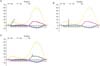
While the knee joint was being flexed approximately 15° during the loading response, the tibia was externally rotated around the femur. We authors first designated it as the 'paradoxical screw-home movement.' The measured angle was approximately 6° (Fig. 4A) using the SKB program. This amount of tibial rotation was maintained during the mid-stance phase (Fig. 4B). As rapid flexion of the knee joint occurred in the pre-swing phase, the tibia started to rotate internally around the femur (a reversal of the screw-home movement). Internal rotation was maintained until it reached peak knee flexion in the initial swing phase. As the knee reached full extension in the lateswing phase, the tibia was rotated externally by 17° (Fig. 4C); thus, it almost reached the neutral position (screw-home movement).
DISCUSSION
The principal findings of this study were that while the knee joint was flexed approximately 15° during the loading response, the tibia was externally rotated around the femur about 6°. The screw-home movement in the tibiofemoral joint occurred due to the unique anatomical shape.16) During the last 20° of knee extension, anterior tibial glide persists on the tibial medial condyle because its articular surface is longer than that on the lateral side. Prolonged anterior glide on the medial side produces external tibial rotation, the screw-home mechanism. When the knee begins to flex (0° of extension to 20° of flexion), posterior tibial glide begins first on the longer medial condyle, and produces relative tibial internal rotation, a reversal of the screw-home mechanism.
When the knee joint is extended, the anterior and posterior cruciate ligaments get tangled and tightened if the tibia is rotated externally with respect to the femur (screw-home movement). Consequently, the knee joint becomes locked in a position; the tibia becoming more stable as compared to the femur. Therefore, the screw-home movement stabilizes the knee joint in the extended position. Many authors have primarily assessed the screw-home movement statically during passive flexion-extension of the knee joint, and little has been studied dynamically during normal gait.
In this study, we attempted to measure the amount and direction of tibial rotation with respect to the femur during gait using optical tracking system and software. Tibial rotation in the transverse plane during gait does occur to a lesser degree than the amount of flexion-extension in the sagittal plane. Therefore, measurement of tibial rotation using conventional gait lab tools has been considered to be not very accurate compared to measurement of flexion-extension. In this study, tibial rotation during gait was measured using additional markers and SKB software to directly compare the rotation angles between the femur and the tibia.
During normal gait, the tibia was expected to rotate internally (a reversal of the screw-home movement) while the knee started to flex during the loading response and in the pre-swing phase. Conversely, the tibia was expected to rotate externally (screw-home movement) as the knee started to extend in the late-swing phase. In this study, as measured using the SKB program, the screw-home movement occurred as expected during the pre-swing phase and the late-swing phase (the open chain movement) of the gait cycle.
However, in this study, the tibia rotated externally with respect to the femur, rather than internally, while the knee joint started to flex during the loading response (closed chain movement). This was the paradoxical screw-home movement that reversed the geometry of contacting joint surfaces, and it may use the energy to internally rotate the femur on the tibia fixed on the ground to provide stability to the knee joint during the remaining stance phase. This is believed to be one of the energy-saving mechanisms of gait, as less energy is used for knee joint locking during the double support period than during the single support period.1617)
Kozanek et al.17) studied the 3D gait analysis and reported that the tibia showed external rotation during the early stages of stance phase as the knee joint started to flex during walking, which was similar to the finding of this study. Qi et al.18) also published similar results. Koo and Andriacchi19) implied that the knee joint mechanics might differ depending on the movement condition by suggesting that the axis of knee joint rotation shifted laterally during gait unlike in the non-weight-loading state.
In this study, the amount of tibial rotation was measured using the SKB program to be about 6° during the loading response and 17° in the pre-swing and late-swing phases. Karrholm et al.20) reported that the rotational movement of the tibia ranged from 9.9° (internal rotation) to 1.6° (external rotation) during the active extension movement of the knee joint among healthy people using the roentgen stereophotogrammetric analysis method. In addition, Lafortune et al.21) conducted a study by inserting the intra-cortical traction pins into the tibia and femur, and they reported that during the stance phase, the tibiofemoral joint exhibited no external rotation, and during the swing phase, external rotation was about 4°. This difference in the range of the rotational movement might be due to the difference in the loads applied to the knee joint, the difference in the measuring tools, and the accuracy of the measurement method. Therefore, a careful analysis of such study results is required.
The 3D gait analysis using optical tracking system allows quantitative and non-invasive measurement of the joint movement during the actual gait cycle. The kinematic analysis of the tibiofemoral joint can be conducted for three rotational movements (internal/external rotation, varus/valgus, and flexion/extension) and three translational movements (anterior/posterior translation, medial/lateral translation, and vertical compression/distraction).20) Measuring these knee movements during gait might provide useful information to assess different morbid gait patterns as well as to determine the efficacy of treatments including surgical reconstruction and rehabilitation. More cases are needed to enhance the statistical power.
For measuring the rotational movement between the tibia and the femur in this study, additional markers were attached, in addition to the Helen-Hayes marker set, to the medial and lateral condyles of the femur and tibia. However, the markers attached to the inner side of the thigh and leg caused the subjects to walk with the hip in 3° of abduction so that the internal markers would not come in contact with each other. This might have interfered with comfortable gait. However, these markers enabled direct measurement of the rotation angle between the femur and the tibia. This could be a limitation of this study. We think that this difference was due to a compensatory mechanism during gait in order to provide a clear space for the markers attached to the inner side of the lower limbs.
This is the first study to measure the direction and degree of the screw-home movement during gait of a normal person by utilizing the optical tracking device. As a result, the screw-home movement occurred in the normal direction in the pre-swing and late-swing phases; however, the paradoxical screw-home movement occurred during the loading response phase. This may be an important mechanism that provides stability during the remaining stance phase. Obtaining standardized values of the knee joint during gait using 3D motion capture analysis can be useful in diagnosing and treating the pathological knee joints.
 XML Download