

 PDF
PDF ePub
ePub Citation
 Print
Print


INTRODUCTION
MATERIALS AND METHODS
Preclinical phantom imaging
Table 1
Acquisition Parameter Settings for Reference Scan and Parameters for All Other Scans in the Phantom Study, Using 3D FSE-Cube Imaging with 1.5T MRI
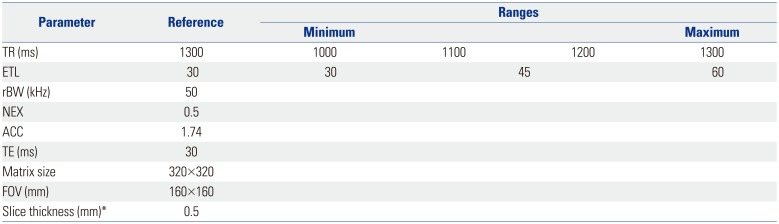
| Parameter | Reference | Ranges | |||
|---|---|---|---|---|---|
| Minimum | Maximum | ||||
| TR (ms) | 1300 | 1000 | 1100 | 1200 | 1300 |
| ETL | 30 | 30 | 45 | 60 | |
| rBW (kHz) | 50 | ||||
| NEX | 0.5 | ||||
| ACC | 1.74 | ||||
| TE (ms) | 30 | ||||
| Matrix size | 320×320 | ||||
| FOV (mm) | 160×160 | ||||
| Slice thickness (mm)* | 0.5 | ||||
3D FSE-Cube, three-dimensional fast spin-echo; TR, repetition time; ETL, echo train length; rBW, receiver bandwidth; NEX, number of excitations; ACC, acceleration factor; TE, echo time; FOV, field of view.
*0.5-mm-slice-thickness isovoxel imaging was reformatted with interpolation after 1.6-mm-slice-thickness scanning.
![]()
Phantom imaging evaluation and selection of optimized parameters
Imaging of patients
Table 2
Acquisition Parameter Settings for Routine Knee MRI of Patients
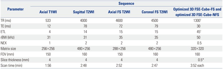
TR, repetition time; TE, echo time; ETL, echo train length; rBW, receiver bandwidth; NEX, number of excitations; FOV, field of view; T1WI, T1-weighted imaging; T2WI, T2-weighted imaging; 3D FSE-Cube-FS, three-dimensional fast spin-echo with fat suppression; 3D FSE-Cube-NFS, three-dimensional fast spin-echo without fat suppression.
*0.5-mm-slice-thickness isovoxel imaging was reformatted with interpolation after 1.6-mm-slice-thickness scanning, †Optimized parameters were results from preclinical phantom study.
![]()
Review of patient imaging
Statistical analysis
RESULTS
Scan parameter optimization by phantom imaging
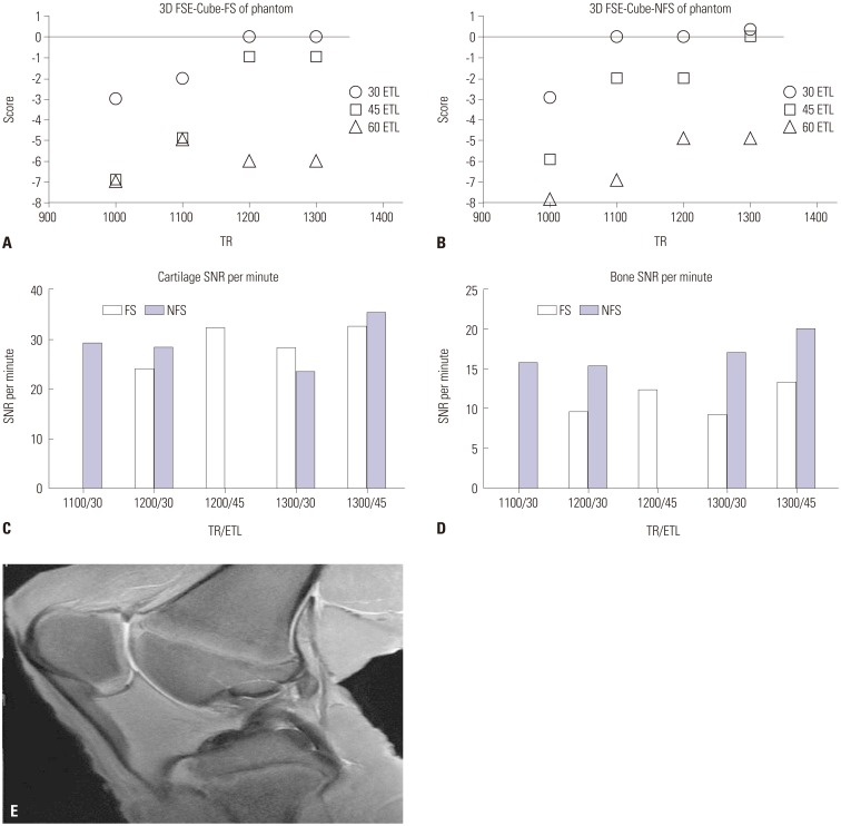 | Fig. 1Subjective scores of phantom imaging (A) with fat suppression and (B) without fat suppression. Images with a score of -1 or above were regarded as acceptable. Highest SNRs per unit time were acquired with scan parameters of TR=1300 ms and ETL=45 in both FS and NFS images with parameter settings of acceptable image quality, measured in the (C) patellar cartilage and (D) femoral epiphyseal bone marrow. (E) 3D FSE-Cube-NFS phantom image with optimized parameters. 3D FSE-Cube-FS, three-dimensional fast spin-echo with fat suppression; 3D FSE-Cube-NFS, three-dimensional fast spin-echo without fat suppression; SNR, signal-to-noise ratio; TR, repetition time; ETL, echo train length.
|
Interpretation of patient imaging
Table 3
Diagnostic Performance of 3D FSE-Cube-FS and 3D FSE-Cube-NFS for Detection of Knee Joint Lesions
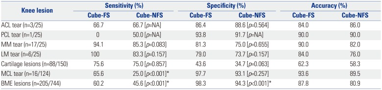
3D FSE-Cube-FS, three-dimensional fast spin-echo with fat suppression; 3D FSE-Cube-NFS, three-dimensional fast spin-echo without fat suppression; ACL, anterior cruciate ligament; PCL, posterior cruciate ligament; MM, medial meniscus; LM, lateral meniscus; MCL, medial collateral ligament; BME, bone marrow edema; NA, not applicable.
Figures represent combined data from independent reviews of the two readers; data in brackets are p-values for comparison of the two imaging techniques.
*p<0.05 indicates a significant difference.
![]()
Table 4
Sensitivity and Specificity of 3D FSE-Cube-FS and 3D FSE-Cube-NFS for Detection of Cartilage Lesions
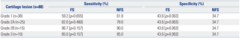
![]()
Table 5
Interobserver Agreement Rates with Unweighted Kappa
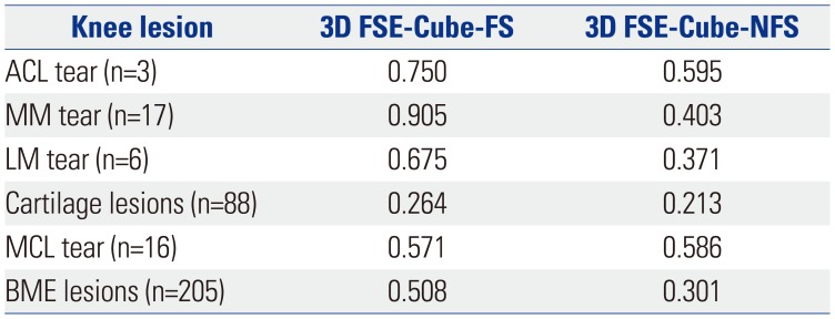
3D FSE-Cube-FS, three-dimensional fast spin-echo with fat suppression; 3D FSE-Cube-NFS, three-dimensional fast spin-echo without fat suppression; ACL, anterior cruciate ligament; MM, medial meniscus; LM, lateral meniscus; MCL, medial collateral ligament; BME, bone marrow edema.
Data represent k-values.
![]()
DISCUSSION
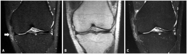 | Fig. 2(A) Blurring of MCL fibers in addition to an increase in signal intensity of surrounding soft tissue are seen on the coronal reformatted 3D FSE-Cube-FS image (arrow). (B) Blurring of ligament fiber is not definite, and no signal abnormality in surrounding soft tissue is detected on the coronal reformatted 3D FSE-Cube-NFS image. (C) Conventional 2D coronal T2-weighted image reveals MCL tear. MCL, medial collateral ligament; 3D FSE-Cube-FS, three-dimensional fast spin-echo with fat suppression; 3D FSE-Cube-NFS, three-dimensional fast spin-echo without fat suppression.
|
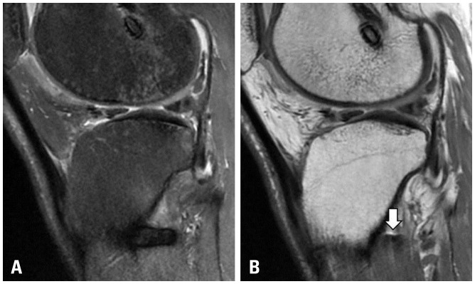
 | Fig. 3(A) 3D FSE-Cube-NFS image shows a suspicious subchondral BME lesion on the posterolateral tibial plateau (arrow), while (B) 3D FSE-Cube-FS image shows a subchondral sclerotic change. After correlation with 2D imaging, it turned out to be a false-positive lesion. 3D FSE-Cube-FS, three-dimensional fast spin-echo with fat suppression; 3D FSE-Cube-NFS, three-dimensional fast spin-echo without fat suppression; 2D, two-dimensional.
|
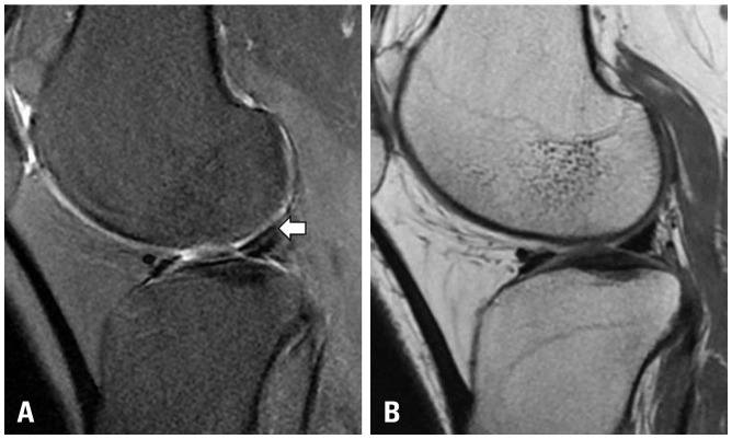
 | Fig. 4(A) Metal artifact posterior to the proximal tibial cortex in 3D FSE-Cube-FS image. (B) Greatly reduced artifact is noted in 3D FSE-Cube-NFS image (arrow). Posterior tibial cortex margin is well-demarcated in this sequence. 3D FSE-Cube-FS, three-dimensional fast spin-echo with fat suppression; 3D FSE-Cube-NFS, three-dimensional fast spin-echo without fat suppression.
|
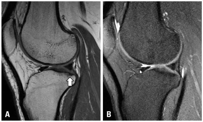
 | Fig. 5(A) Artifact during 3D FSE-Cube-FS imaging. It is impossible to know whether there is a tear in the LM (arrow). (B) Subsequent 3D FSE-Cube-NFS image shows a normal meniscus. 3D FSE-Cube-FS, three-dimensional fast spin-echo with fat suppression; 3D FSE-Cube-NFS, three-dimensional fast spin-echo without fat suppression; LM, lateral meniscus.
|
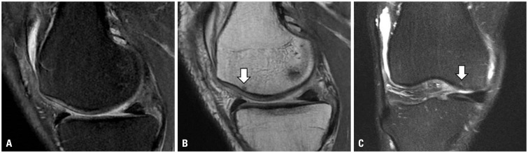 | Fig. 6(A) No definite subchondral bone marrow signal change is seen in the medial femoral condyle in 3D FSE-Cube-FS image. (B) A small suspicious low signal intensity lesion is seen in the subsequent 3D FSE-Cube-NFS image (arrow). (C) Conventional 2D coronal T2-weighted image reveals a tiny subchondral BME lesion in the medial femoral condyle (arrow). 3D FSE-Cube-FS, three-dimensional fast spin-echo with fat suppression; 3D FSE-Cube-NFS, three-dimensional fast spin-echo without fat suppression; 2D, two-dimensional.
|
 XML Download