

 PDF
PDF ePub
ePub Citation
 Print
Print


INTRODUCTION
Hemodialysis is widely used to treat end-stage renal failure. With the development of hemodialysis and artificial biomaterial technology, the efficiency of dialysis has increased rapidly, reducing the time required for dialysis and lengthening the average lifespan of patients. However, the main complications of hemodialysis have not yet been fully resolved, and they include hypotension and osmotic disequilibrium syndrome. Hypotension occurs as a result of the rapid reduction in blood volume caused by ultrafiltration, whereas the main cause of osmotic disequilibrium syndrome is the osmotic disequilibrium between the inside and outside of cells due to the change in plasma solute concentrations, which leads to excessive fluid transfer.
Optimum dialysate composition and ultrafiltration rate for dialysis are calculated by evaluating physiological changes in blood pressure, body temperature, and electrolyte balance. In practice, a mathematical model of the physiological system has usually been used to evaluate physiological changes in dialysis patients. Any numerical model of the dialysis process should precisely predict physiological changes of patients and optimal dialysate composition.
There are several mathematical models of dialysis systems. Kimura et al.1 used trans-capillary and trans-cellular models to numerically interpret the change in plasma volume, Ziolko et al.2 analyzed the changes resulting from the complexity of dialysis and mass transfer models, and presented data on the precision and efficiency of the data. Akcahuseyin et al.3 explained the decrease in blood volume that occurred during dialysis using a model of mass transport among compartments and revealed that fluid transportation resulting from an uneven electrolyte distribution among cells is a crucial factor affecting blood volume. To explain the transport of fluids and solutes through cell membranes and vessel walls during hemodialysis, Ursino et al.4 used a mathematical bio model consisting of 3 compartments: intracellular fluid, interstitial fluid, and plasma.
Although the existing dialysis models primarily explain transactions among cells, extracellular fluids, and plasma during dialysis from a local perspective, the only modeling study to consider the global cardiovascular hemodynamics is that by Ursino et al.5 They combined the interpretation method of the 3 compartment dialysis model with a simple cardiovascular system model and autonomic control function in an attempt to explain cardiovascular changes resulting from dialysis. Unfortunately, this model consists of 8 components that greatly simplified the cardiovascular system, therefore, it could not predict dialysate transport through the AV shunt and superior vena cava. In addition, the model assumed that only 1 type of tissue circulation existed and ignored the distribution of blood flow to the upper and lower parts of the body and viscera. Furthermore, the short-term autonomic control function, which is the core of the reaction of the cardiovascular system to dialysis, was expressed using a very simple control model that applied a proportional differential (PD) method. However, as shown by DeBoer et al.,6 the human short-term autonomic control function accommodates not only beat-to-beat characteristics related to heart beat but also is intimately related to the characteristics of sympathetic and parasympathetic nerve conduction.
Herein, we developed an improved numerical simulation code that explains cardiovascular response during dialysis and estimates optimal composition of the dialysate. Unlike existing models, ours considers detailed hemodynamic factors based on anatomic characteristics, including the movement of blood through the AV shunt and superior vena cava for dialysis. Our model also incorporates a short-term autonomic control function that applies an improved method for incorporating the beat-to-beat mechanism of the autonomic control function and sympathetic and parasympathetic nerve conduction. Our method is a detailed model that includes a 2 compartment solute kinetics model, 3 compartment body fluid dynamic model, 12 compartment cardiovascular system model, and baroreflex autonomic control function. Using this model, we can simulate the changes in response of a patient's cardiovascular system during hemodialysis.
We evaluated the precision and validity of our model by comparing the results with those of existing dialysis models, and used our model to investigate cardiovascular response to different Na+ concentration profiles. After evaluating the results, the profile found to be most efficient for preventing hypotension and disequilibrium syndrome during dialysis is presented.
MATERIALS AND METHODS
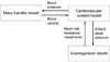
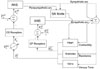
To evaluate cardiovascular response to dialysis, we created a numerical evaluation system that combined existing models (Fig. 1), including a model of mass and volume transport during dialysis, cardiovascular hemodynamic system model, and autonomic control function model. The lumped parameter model proposed by Ursino et al.4 was used as the mass and volume transport model, and the multi-branched lumped parameter hemodynamics model and the beat-to-beat method baroreceptor reflex model proposed by Heldt et al.7 were used for cardiovascular system and autonomic control function, respectively.
Mass transport model
The mass transport that occurs during dialysis can be roughly explained using body fluid exchange and solute kinetics as in the model of Ursino et al.5 Body fluid compartments can be approximately classified into intracellular and interstitial fluid and plasma compartments. Intracellular and interstitial fluid exchange usually occurs as a consequence of osmotic differences that arise at the cell membrane due to differences between solute concentrations inside and outside the cell. Fluid exchange between interstitial fluid and plasma arises from differences between oncotic and hydrostatic pressure. Proteins generate an osmotic pressure difference between plasma and interstitial fluid, and this difference participates in the fluid exchange between interstitial fluid and plasma. This pressure, called "oncotic pressure", was calculated using the Landis-Pappenheimer equation. Furthermore, assuming that the elastic coefficient of tissues is constant, hydrostatic pressure of the interstitial fluid was calculated as a function of interstitial fluid volume and elastic coefficient of tissues.5 The movement of solutes into and out of cells provides the main mechanism of diffusion and involves both passive channels and active pumps.
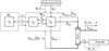
Fig. 2 is a schematic diagram of the mass transport model used in this study. The solid lines show the exchange of fluids and the dotted lines show the transport of solutes. Ms,ic and Ms,ex represent the mass of solute s inside and outside the cell, respectively; the mass transport coefficients for this solute from the inside and outside of the cell are ηs and ηs·βs, respectively. βs is an equilibrium ratio that sets the ratio cs,ic/cs,is at the state of the resting potential through the cell membrane. The model considers the solute urea, creatinine, Na+, K+, and HCO3-. Vic, Vis, and Vpl are the volumes of intracellular fluid, interstitial fluid, and plasma, respectively, and the extracellular volume Vex is the sum of Vis and Vpl. Qinf and Qf are the substitute fluid injection and ultrafiltration rate, respectively, and Cs,inf is the solute concentration dissolved in the substitute fluid. Js is the transport rate of the solutes through the dialyzer, and Fa(t) and Rv(t) are the plasma filtration of arterial capillaries and reabsorption rate of venous capillaries, respectively. The plasma filtration and reabsorption rates are calculated using equations (6)-(9). While Ursino et al.4 assumed constant arterial and venous capillary pressures, we assumed that arterial and venous capillary pressure were not constant and used time-varying values from Heldt et al.7: Pac1 as Pup, Pac2 as Psp, Pac3 as Pll, Pvc1 as the difference between Pup and Psvc, Pvc2 as the difference between Psp and Pavc, and Pvc3 as the difference between Pll and Pavc. By coupling dependent variables in the cardiovascular system model with time-varying parameters in the mass transport model, the integrated model achieves more realistic results. Water permeability through the cell membrane is represented by ηf.
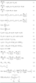
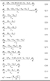
The governing equations for the mass transport model used in the actual numerical calculations are listed in Appendix 1.
Cardiovascular system model
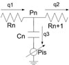
A cardiovascular system model using a lumped parameter method was used to evaluate the cardiovascular system. Using components to express the crucial factors that participate in blood circulation, this model calculates pressure and volume at each component along with blood flow among components. Owing to conceptual similarities, this model can easily be represented by using electric circuit diagrams. Fig. 3 shows a representative component in which blood flow corresponds to electric current and blood pressure corresponds to voltage. Electric resistance expresses flow resistance inside blood vessels due to viscosity, and the storage battery is equivalent to the compliance of blood vessel walls. Therefore, changes in the state of a discretionary component are expressed by using the blood flow resistance (R) at the entrance and exit to the component, capacitance (C), blood flow (q), blood pressure (P), and pressure acting on the exterior wall of the blood vessels (Pis), which is calculated in the above model as a function of interstitial fluid volume and elastic coefficient of tissue. To facilitate interpretation, all resistance elements and storage batteries were assumed to be linear elements.
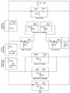
Based on earlier research and anatomic information, we expressed all human blood flow relationships using a simplified closed circuit consisting of 12 components (Fig. 4): the left ventricle (lv), aorta (a), right ventricle (rv), pulmonary artery (pa), pulmonary vein (pv), and components of the tissue circulation system, including 3 parts of the vena cava-the superior vena cava inside the thoracic cavity (svc), inferior vena cava inside the thoracic cavity (ivc), and vena cava outside the thoracic cavity or abdominal vena cava (avc) and 4 arterial branches: the upper body (up), kidney (kid), splanchnic organs (sp), and lower limb (ll). The contraction and relaxation of the heart to serve its pumping function used a predetermined value that changed with time. More detailed information is available in the study by Heldt et al.7 The effect of the atrium is only as an accessory, therefore, it was included in the calculations of adjacent nodes. Diodes at the entrances and exits of ventricles represent the heart valves that prevent blood reflux. Pressure that changes with time, Pth, is the pressure in the thorax. In addition, exterior pressure affecting a vessel is indicated by the subscript is, which means interstitial. Finally, ultrafiltration rate is Qf, injecting flow rate of the substituting fluid is Qinf, and the difference between the 2 values equals the actual volume change of the plasma through the dialyzer. To express the actual phenomenon more accurately, this dialysis component was located at the wrist (the cephalic vein), where the AV shunt is. The governing equations of the 12-parameter model of the cardiovascular system are given in Appendix 2.
Autonomic nerve control model
When the cardiovascular system is disturbed and components such as arterial pressure are altered, the autonomic nervous system (ANS) performs several control functions. First, average arterial blood pressure (PA) is sensed through baroreceptors in the carotid sinus artery. This information is transmitted to the ANS, where an error signal for the difference between the transmitted pressure and standard value is generated. This signal is transmitted to various cardiovascular components via sympathetic and parasympathetic nerves, changing the heart rate at the SA node and increasing or decreasing heart contractility by changing the calcium concentration inside cardiac myocytes. Furthermore, alteration of the contractility of vascular smooth muscle regulates vascular resistance and venous tone. This series of processes forms a feedback control system to restore the blood pressure changed (error signal) sensed in the carotid artery to normal.
We used a baroreceptor reflex model based on a beat-to-beat method (Fig. 5) to mimic the response of the human autonomic control function to the short-term disturbance of the cardiovascular system caused by dialysis. PA represents the average arterial pressure that is a substitute for carotid artery pressure, and is a variable input to the system. The effective pressure deviation (PAeff) sensed by the autonomic nervous system can be expressed by the equation (32), as given by DeBoer et al.6
This nonlinear equation expresses the tested observation that the error signals are not amplified by the neural system in response to an excessive percentile range in pressure. Any significant pressure percentile range is transmitted through sympathetic and parasympathetic nerves. However, because the transmission speed differs between the 2, the stimulus-reaction curves also differ, such that the response time of the parasympathetic nerve is fast (0.5 - 1 s) and that of the sympathetic nerve is slow (3 - 10 s). This model, developed by DeBoer et al.6 for the command transmission of autonomic control function, was successfully introduced in studies by Heldt et al.7 and Shim et al.8 The ganglion transmission model and autonomic control function used here have thoroughly been discussed in a review by Shim et al.9
It is known that disturbances of ANS function are common in chronic renal failure (CRF) patients and its mechanism is multifactorial. Reduced end-organ response to norepinephrine appears to be a major factor underlying these abnormalities in CRF patients. Derangements in the parasympathetic nervous system and/or disturbances in cardiac function may also be involved.10 However, there are few quantitative data on the variations of cardiovascular variables such as heart rate and arterial resistance according to ANS disturbance. Because of this reason, we did not consider the ANS disturbance during hemodialysis, which may be one of the main limitations of the present study.
Sodium ion (Na+) concentration profile
A dialysate with a constant Na+ concentration is usually used for dialysis treatment. However, in patients requiring dialysis of a large volume of blood, a dialysate with a Na+ concentration that changes over time is used to slow Na+ exchange in the body.6 In these cases, Na+ concentration in the extracellular fluid decreases rapidly at later dialysis times. Therefore, the change in Na+ concentration with time is represented by an upwardly convex curve. In clinical tests, Ursino et al.11 verified that the rates of intracellular and extracellular volume changes could be reduced in patients using this method.
In the present study, we wanted to predict how the exchange rate of a patient's intracellular and extracellular volume and cardiovascular response change during the course of dialysis as a function of the Na+ concentration profile. Thus, we evaluated 3 profiles: (1) a convex downward profile, (2) convex upward profile, and (3) linear profile intermediate between the two. By comparing cardiovascular response in these 3 cases, we expected to predict physiological effects of plasma Na+ concentration profile on the cardiovascular system and determine the optimal Na+ profile based on a patient's characteristics.
Initial conditions and numerical parameters
The values of the basic parameters and initial conditions of the numerical model that were used to investigate cardiovascular system response during hemodialysis were estimated from general conditions in dialysis patients. For an average adult with a body weight of 70 kg, hemodialysis is performed for 4 hours and involves about 2 L of fluid at an ultrafiltration rate of 0.5 L/hr. The overall mass transfer coefficient, KoA, of the simulated dialyzer is 700. The other parameters and initial conditions used in the models were obtained from Ursino et al.11 and Heldt et al.7
RESULTS
Validating the material transport and cardiovascular system model
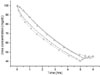
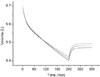
To validate the mass transport model in terms of body fluid exchange and solute transport, the calculated results were compared to the results of Barth et al.,12 which assumed a constant body fluid and used a 2-compartment model to calculate urea concentration profile. To facilitate the comparison, we used a urea clearance rate identical to that used by Barth et al.,12 As shown in Fig. 6, the 2 models give essentially identical urea concentration profiles and both show the concentration rebound phenomenon for extracellular fluid. In the study by Barth et al.,12 urea concentration in extracellular fluid decreased from an initial value of 100 mg/dL (the BUN in a chronic renal failure patient) to 40 mg/dL after 5 hrs of dialysis and then increased by 5 mg/dL after an additional hr. In our study, the concentration decreased to about 37 mg/dL and then rebounded by about 5 mg/dL after 1 hour.
The mass transport model
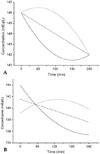
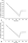
The results of the 3 different dialysate Na+ concentration profiles calculated using the inverse algorithm are shown in Fig. 8B. Inversely, we used the dialysate Na+ concentration profile in the model to determine the above plasma Na+ concentration profile (Fig. 8A). In profile A, it decreases rapidly, but the rate of decrease slows down after 2 hours and then increases to a concentration of 142 mEq/L after 3 hours. In profile B, the concentration decreases at a constant rate. In profile C, the plasma Na+ concentration increases for a short period early in dialysis, decreases gradually after about 1 hour, and then decreases rapidly after 2 hours to 142 mEq/L.
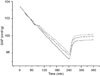
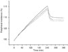
Fig. 9 shows the temporal changes in overall blood volume according to Na+ concentration profile. The calculation time was set at 6 hours, consisting of 4 hours of dialysis and 2 hours of observation after dialysis. Although the differences among blood volumes are not large, they increased according to the profile in the order A < B < C. For profile A, the blood volume is minimized while for the opposite case, i.e., profile C, the blood volume is maximal. Profile B has a blood volume intermediate between the two.
Cardiovascular system response during hemodialysis
The physiological response of the cardiovascular system and autonomic nervous system to hemodialysis were evaluated. Again, the calculations were for a 6-hour period, reflecting 4 hours of hemodialysis and 2 hours of observation.
Fig. 10 shows the temporal variation in systemic arterial pressure (SAP). Under autonomic nervous system control, arterial pressure decreased linearly to 96 mmHg. Among the 3 different Na+ concentration profiles, SAP at the end of the dialysis session, decreased the most with profile A and least with profile C.
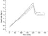
Fig. 11 illustrates the temporal change in heart rate. Heart rate increased at an almost constant rate of 1.5 bpm per hour over 4 hours of dialysis. After dialysis, heart rate decreased gradually but remained markedly elevated 2 hours after dialysis. Consequently, comparing heart rate and sodium concentration, heart rate was greatest with profile A, lower with B, and lowest with C.
Fig. 12 shows temporal change in systolic compliance of the left and right ventricles during dialysis. Although the right ventricle is more compliant than the left, both ventricles had the lowest compliance with profile A and the highest with C.
Fig. 13 shows the percentage change in total peripheral resistance, which consists of resistance in the lower limbs, splanchnic organs, and upper body compartment. During hemodialysis, peripheral resistance increased by about 15%. On comparing profiles, the magnitude of resistance was in the order A > B > C.
DISCUSSION
This study presented a numerical simulation model for estimating cardiovascular response in dialysis patients during sodium-profiled hemodialysis. The model is a complex one that consists of cardiovascular, ANS, and mass transport models. These models make it possible to estimate cardiovascular system response during profiled-hemodialysis, reaction of the ANS, and diverse reactions concerning the dynamics of body fluid exchange and solute transport.
As discussed in the section on sodium ion (Na+) concentration profile, when considering the 3 plasma Na+ concentration profiles of dialysis patients (Fig. 8A: profile A; convex downward, profile B; linear reduction, and profile C; convex upward), temporal change in Na+ concentration of the dialysate used to induce plasma Na+ concentration was calculated using an inverse algorithm (Fig. 8B). The target plasma Na+ concentration profile had been established in advance, and the Na+ concentration profile of the injected dialysate was calculated by applying this value to the inverse algorithm.
In the treatment following profile A, the convex downward curve maintains a low plasma Na+ concentration in the middle of the treatment because of the low dialysate Na+ concentration profile. Therefore, plasma osmolarity falls below interstitial fluid osmolarity. Arterial capillary filtration increases more than venous reabsorption. Finally, plasma volume decreases during treatment (Fig. 9). With treatment using profile C, the convex upward curve makes plasma volume decrease least among the 3 profiles because it has the highest dialysate Na+ concentration profile.
As plasma volume decreases, SAP decreases proportionally. Then, the ANS makes HR and peripheral resistance increase and systolic compliance decrease to maintain a normal SAP. The 3 types of temporal change in heart rate (Fig. 11) show that the ANS responds to arterial pressure reflex differently, according to Na+ concentration profile. Arterial pressure decreased with the loss of blood volume. Therefore, the autonomic nervous reflex is activated to maintain arterial pressure by increasing heart rate. The autonomic nervous baroreflex system maintains arterial pressure around the normal range by increasing stroke volume. Fig. 12 shows that ventricular systolic compliance decreased during treatment, indicating that stroke volume increased. Another mechanism by which the ANS maintains arterial pressure within the normal range is by increasing peripheral resistance. Consequently, profile A, which involved the greatest pressure change, had the highest resistance, and profile C had the lowest resistance (Fig. 13).
The numerical results matched the published results, allowing us to analyzecardiovascular changes associated with the 3 different sodium profiles. An inverse algorithm was used to determine sodium concentration profile in the dialysate that corresponds to a given plasma sodium concentration profile. Comparison of the calculated results for the 3 profiles showed that hypotension was best avoided by gradually changing the sodium ion concentration at the beginning of dialysis and then increasing the rate of change during the later stage of the process (profile C). By conducting numerical tests of dialysis/cardiovascular models for various treatment profiles and creating a database from the results, it should be possible to estimate an optimal sodium concentration profile for each patient. However, one of the main limitations of the present study is that we did not compare the numerical results obtained by using the 3 different sodium concentration profiles of the dialysate with experiments. An experimental evaluation of the cases is planned for a our future study.
 XML Download