

 PDF
PDF ePub
ePub Citation
 Print
Print


INTRODUCTION
Despite substantial progress in therapeutic efforts, the outcome of some malignant cancers remains very poor. Novel therapies are being developed, one of which is a method to suppress cancer angiogenesis that was proposed by Folkman1 and others.
There have been many modeling studies of tumor angiogenesis in which continuous or discrete models were used. In continuous models, only the distribution of enthothelial cells is considered; vascular networks are not included. Chaplain et al.2,3 presented two- and three-dimensional models of tumor angiogenesis using a combination of both the discrete and continuous method. To determine the movement of the sprouting tips of enthothelial cells, the authors solved partial differential equations of the concentration of a tumor angiogenesis factor (TAF), fibronectin concentrations, and endothelial cell density using the finite difference method. The formation and growth of vessel sprouts were approximated using a stochastic process that was based on the distribution of TAF and fibronectin. Chaplain et al.2,3 also assumed that TAF secretion was constant over time. The numerical solutions of such models can be compared to experimental data, and cellular mechanisms can be incorporated readily into new mathematical models. Lastly, Gazit et al.4 used fractal theory to compute the vessel networks that surrounded a tumor and computed the hemodynamics within the vessel structures.
MATERIALS AND METHODS
Previous works
Recently, Tong et al.5 developed a two-dimensional model of angiogenesis in which they assumed a biased random motion of endothelial cells. To obtain basic information about the biased growth of endothelial cells, the authors examined the transport of angiogenic factors in rat cornea. Because vessel growth in their study was independent of the computation mesh (unlike Chaplain's model), tumor angiogenesis was implemented in a more realistic and efficient manner. However, one of the main problems with previous models is that the quantity of angiogenic factors that are released from tumor cells is assumed to be constant. This assumption is unrealistic because as the volume of a tumor increases, the quantity of angiogenic factors that are released also increases.
In the present study, we present a computational model of tumor-induced angiogenesis for a growing brain tumor, based on Tong's model.5 However, in contrast to Tong's and other models, our model includes dynamic (time-varying) release of angiogenic factors from tumor cells. The model of the growing brain tumor that we used was adopted from the work of Kansal et al.6 The quantity of TAF released from a growing brain tumor depends on the volume of the tumor and the number of constituent cells. We selected basic fibroblast growth factor (bFGF) as a TAF, because the concentration of bFGF is reportedly proportional to the increase in malignancy and vascularity of high-grade gliomas.7,8 Some parameter values for bFGF-induced angiogenesis were obtained from Tong et al.,6 and we used 50 pg/105 cells per 24 h as the production rate for bFGF by human U87 glioma cells.9 The finite element method was used to solve the convection-diffusion equation for the concentration of bFGF. This method is a convenient way with which to deal with the complex geometry of real biological phenomena. Both vessel formation and sprout elongation were simulated using a stochastic process as in the aforementioned studies.
Model
Algorithm
Transport equation for basic fibroblast growth factor
The transport of bFGF within tissue depends on the diffusion of this molecule into the interstitial space, uptake of bFGF by endothelial cells, and chemical inactivation of bFGF within the extracellular space. The partial differential equation of bFGF transport is represented in Eq. (1), which was obtained from Tong et al.5
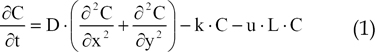
In Eq. (1), C, D, k, u, and L represent the concentration of bFGF, the diffusion coefficient of bFGF, the rate constant of bFGF degradation, the rate constant of bFGF uptake, and vessel density (defined as the total vessel length per unit area), respectively. For the computational domain, application of the Galerkin finite element discretization for Eq. (1) yielded the following matrix equation.
KX=R (2)
In this matrix, K is the stiffness matrix, X is the vector of unknown nodal variables of C, and R contains the external driving forces. The matrix Eq. (2) was solved using an incomplete conjugate gradient method.10
Sprout formation and elongation
The initial response of the endothelial cells to bFGF is chemotactic, and this initiates the migration of endothelial cells towards the bFGF-releasing tumor. Thereafter, small capillary sprouts are formed. The sprouts increase in length owing to the migration and recruitment of endothelial cells. The sprouts continue to grow towards the growing tumor, guided by the motion of the leading endothelial cell at the tip of the sprout.
First, we introduced a threshold function f(C) to account for the effect of concentration of bFGF on sprout formation and elongation, as follows.
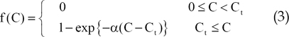
In Eq. (3), Ct is the threshold concentration and α is a constant that controls the shape of the curve.
To approximate sprout formation, we assumed it to be a stochastic process. The probability n for the formation of one sprout from a vessel segment in a time interval between t and t+Δt is proportional to Δt, the segment length Δl, and the threshold function, as follows:
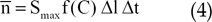
In Eq. (4), Smax is a rate constant that determines the maximum probability of sprout formation per unit time and vessel length.
The growth of a sprout is determined by the locomotion of its tip, while the geometry of a sprout depends on the tip trajectory.10 The direction of sprout growth at each time step depends on two unit vectors: the direction of growth in the previous time step and the direction of the concentration gradient of the angiogenic factors. This is because sprout growth depends on endothelial cell migration, which has a tendency to persist in the same direction as in the previous time step. To reflect the effect of the extracellular matrix on cell migration, we assumed that the angle of deviation, θ, was between 90° and -90° and that tan had a Gaussian distribution with a mean of zero and a variance of σ2. A detailed description of sprout formation and elongation can be found in the reference.5
Brain tumor growth model
We used a model of a brain tumor that had four distinct growth stages, namely spherical, detectable lesion, diagnosis, and death.6 To approximate data in each of these growth stages, we used the following Gompertz equation:
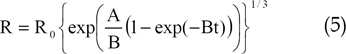
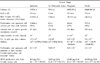
In Eq. (5), A and B are parameters and is the initial volume. The quantity of bFGF release at each of the four stages is summarized in Table 2. We assumed that tumor growth was spherical and investigated a 1.0-mm-thick, circular slice of the tumor for our two-dimensional model. As both the proliferative and quiescent tumor cell fractions likely release bFGF, we calculated the amount of bFGF at each of the four stages for the total amount of living tumor cells using the cell numbers reported by Kansal et al.6
Analysis
Two-dimensional simulation model
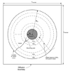
The two-dimensional model is depicted in Fig. 1. In Fig. 1, Ldomain, RPV and Rt represent the distribution of bFGF, the radius of the parent vessel measured from the center of the tumor, and the tumor radius, respectively. We assumed that the radius of the tumor increased over time and calculated the tumor radius using Eq. (6).
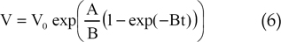
In Eq. (6), R0 was assumed to be 1.0 mm as an initial condition. RPV was selected to allow the first branch to reach the source at a time point at which the tumor radius was 1.0 mm.11 We found that a lattice disk with a radius of 4.5 mm satisfied this condition, and Ldomain was assumed to cover the disc. We also assumed that bFGF was released continually from the tumor, which was located at the center of the aforementioned disk (i.e., represented as a solid circle in a transverse section of the tumor). The region into which angiogenic factors diffused was a 10.0×10.0-mm square (Ldomain=10.0 mm). Three points of initial sprouting were located between 180° and 270°.
Initial and boundary conditions
To solve the equation that governed the concentrations of angiogenic factors (Eq. (1)), a 'no flux' condition was assumed for bFGF transport at the boundary of the diffusion region. The initial concentration of bFGF was zero within the computational region. For computational convenience, we assumed that the initial radius of the tumor was 0.1 mm. The concentration of bFGF at the tumor site increased with the tumor volume, which concurs with a cellular automaton model described previously, in which a growing brain tumor was simulated over several orders of magnitude.6 Table 2 shows the rate of bFGF production over time. For the space discretization of the computational domain, a 200 × 200 finite element lattice was used and linear approximations of the variables within elements were assumed. We calculated both symmetrical and asymmetrical tumor growth.
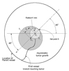
For asymmetrical tumor growth, we assumed that tumor growth was symmetrical before the first vessel branch made contact with the tumor surface; thereafter, growth was assumed to be asymmetrical (see Eq. (7)). As represented in Fig. 2, the vessel branch contacted the tumor surface when R=1.0 mm (T1 tumor with center point C1), after which the tumor began to grow eccentrically. The eccentricity L at time t (T2 tumor with center point C2) owing to asymmetrical tumor growth was defined as follows:
L=(t-tref)Vecc if t > tref (7)
In Eq. (7), t and tref represent the arbitrary time and reference time at which the first vessel branch made contact with the tumor surface, respectively. According to the preliminary computation, tref was -2,600 h. Vecc is a variable that represents the rate of eccentricity change; therefore, the eccentric distance at a time t can be expressed as Eq. (7). In this study, we assumed that Vecc=0.003 mm/h. The direction of eccentricity was 225°. In the equation above, note that only the part of the tumor that was facing the blood vessels grew.
Branching pattern analysis
To quantify the vessel branching pattern within the computational domain, we calculated the number of branching points within a given region of interest (ROI). A ROI was defined as 50 circular areas that divided the space between the central tumor domain and the circle from which the parent vessel originated (see Fig. 1). A branching point was defined as the site at which one vessel was divided into two new vessels (Fig. 1). For each ROI, the total number of branching points within the ROI was calculated according to the average distance of the ROI from the parent vessel. To take into account temporal variation of vessel growth, we considered the total length of vessels at certain time points (equivalent to the sum of the lengths of all vessels that existed at that point in time).
RESULTS
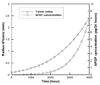
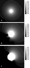
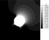
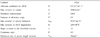
First, we computed a standard case for the parameters as shown in Table 1. Dynamic changes in the tumor radius and the concentration of bFGF (Fig. 3) were computed from Eq. (6). Compared to the tumor radius, the concentration of bFGF had a sharper gradient after t=3,000 h. The concentration distribution over time of bFGF (Fig. 4) revealed that the concentration distribution of bFGF was a radial isotropic gradient at t=1,656 h (spherical state), because the bFGF excreted from the tumor diffused spatially in all directions and only very short branches existed close to the parent vessel. As the branched vessels grew toward the tumor surface, bFGF consumption occurred around these vessels. The radial gradient of the concentration distribution of bFGF ceased to vary isotropically; the concentration of bFGF was very low on the side on which the vessels were growing and was relatively high on the side opposite to the parent vessel (Fig. 4(B) and (C)).
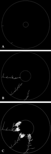
The vessel branching pattern for symmetrical tumor growth is shown in Fig. 5. Initially, three branches from the parent vessel grew toward the tumor following the concentration gradient of bFGF. The lowest branch appeared to be very short initially, but subsequently branched numerous times as it approached the tumor surface. In our simulation, the first vessel branch touched the tumor surface at t=2,590 h; this vessel branching pattern is exemplified by the pattern in Fig. 5(B), which illustrates the branching pattern at t=2,600 h. At t=3,200 h, there were numerous vessel branches close to the tumor surface (the brushborder effect; Fig. 5(C)).
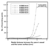
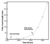
The pattern of vessel growth for symmetrical tumor growth is illustrated in Fig. 6. At t=1565 and t=2600 h, the number of branching points near the tumor surface was largely unchanged, whereas at t=2800 and t=3000 h, there was a marked increase in the number of branching points near the tumor surface. The total vessel length was relatively constant initially, but increased sharply after the first vessel reached the tumor surface at t=2,590 h (Fig. 7).
Asymmetrical tumor growth is illustrated in Fig. 8 and 9. Unlike symmetrical tumor growth, asymmetrical growth was associated with slightly elevated concentrations of bFGF at the tumor surface (Fig. 8), which acted as promoter that enhanced branching of the parent vessel. Nevertheless, the difference in the concentration of bFGF during symmetrical and asymmetrical growth was small. Fig. 9 illustrates that asymmetrical tumor growth was biased toward the parent vessel. Although the pattern of vessel branching was similar to the case of symmetrical growth, branches generated from the lowest location of the parent vessel during asymmetrical growth were more densely distributed close to the tumor surface as compared to during symmetrical growth. Changes in the total vessel length during asymmetrical tumor growth were similar to those that occurred during symmetrical growth, but the total vessel length was slightly greater after t=3,000 h as compared to that during symmetrical growth.
DISCUSSION
In this study we proposed a new computational method to simulate tumor angiogenesis in two dimensions. For the analysis of the spatial distribution of bFGF over time, the bFGF conservation equation was solved using a finite element method. Unlike previous studies, we assumed that the tumor grew over time in our model. This allowed us to observe the effect of dynamic bFGF production and its effect on vessel branching patterns. The brain tumor model proposed by Kansal et al.6 was used as a basis for our model of a growing tumor, which comprised four distinct stages, namely spherical state, first detectable lesion, diagnosis, and death. In the present study, we computed both symmetrical and asymmetrical tumor growth and compared the results of each. Biased tumor growth toward vessel branches was assumed to simulate the asymmetric growth of the tumor.
From a computational aspect, we used a finite element method to solve the conservation equation of bFGF concentrations, whereas a finite difference method was used in previous studies. It is widely recognized that the finite element method is more flexible when dealing with complex geometry. In addition, it is relatively easy to implement boundary conditions with this method. However, the finite element method requires more computing time than the finite difference method. If a realistic tumor geometry obtained from magnetic resonance imaging data is adopted as the computational model, the finite element method is better suited to solving the equations for such a complex shape. If the finite element method that we used is combined with an automatic mesh generation program in a two-dimensional (triangular mesh) or three-dimensional (tetrahedron mesh) geometry, a realistic (and therefore clinically relevant) tumor can be simulated.
Our model is novel in that we simulated a tumor that grew and exhibited angiogenic responses to changing concentrations of bFGF. As shown in Fig. 7, the number of vessel branches increased dramatically as soon as a vessel branch made contact with the tumor surface for the first time. This can be explained physiologically by the fact that tumors generally grow rapidly once blood is supplied to them directly from a parent vessel; therefore, tumors exhibit a bias in growth that is skewed towards the parent vessel. To examine the effect on angiogenesis of such biased tumor growth, we computed a comparison of asymmetrical and symmetrical tumor growth. In the case of symmetrical growth, bFGF was almost completely consumed at the tumor surface. By contrast, there were slightly higher concentrations of bFGF at the tumor surface during asymmetrical growth, which acted as a promoter that enhanced the branching of the parent vessel.

 XML Download