

 PDF
PDF ePub
ePub Citation
 Print
Print


INTRODUCTION
Quantification of the hemodynamic features of blood flow is important because these features are closely related to the development of cardiovascular diseases. Blood flow exerts various types of fluid dynamic forces on the blood vessel, including pressure force and frictional shearing stress. Endothelial cells on the vessel wall sense and respond to these hemodynamic conditions by adapting their morphology and proliferation (1). The pathological hemodynamic forces exerted on the vessel wall consequently induce inflammatory lesions in the vessel that promote the development of atherosclerosis, aortic dilatation, and aortic aneurysm (2345). In addition, the mechanical forces of the blood flow influence plaque vulnerability and the risk of aneurysm rupture (67). Therefore, quantification and understanding of the characteristics of blood flow are important in diagnosing and predicting the future risk of cardiovascular disease.
Time-resolved, three-dimensional (3D) phase-contrast (PC) magnetic resonance imaging (MRI), which is also termed four-dimensional (4D) PC-MRI or 4D flow MRI, was recently developed to investigate spatial and temporal variations in the hemodynamic features of blood flow (89). This technique permits the volumetric assessment of blood flow in the entire vasculature of interest and enables the volumetric quantification and retrospective analysis of blood flow in any arbitrary angle, which is not possible with conventional two-dimensional (2D) PC-MRI.
Based on the volumetric velocity data of 4D PC-MRI, various methods have been developed to visualize and quantify blood flow, and their clinical implications have been studied (10). The visualization of 4D PC-MRI data using vector field, streamline, pathline, isosurface, and volume rendering has been effective in identifying the abnormal alteration of blood flow in various vessels, such as the aorta, carotid arteries, and cerebral vessels (111213). Volumetric acquisition of the blood flow also enables better visualization and quantification of the complex nature of intracardiac blood flow (1415). 4D PC-MRI provides not only the conventional flow quantifications, but also various fluid dynamic biomarkers with potential clinical utility, such as wall shear stress (WSS) (34), turbulent kinetic energy (TKE) (161718), vorticity (1920), pressure gradient (212223), and pulse wave velocity (2425).
The purpose of our present review is to discuss recent advances in 4D PC-MRI. We briefly overview the principles and analytical procedures of 4D PC-MRI, and introduce various fluid dynamic biomarkers that can be obtained using the technique. In addition, we overview the clinical applications of 4D PC-MRI in various cardiovascular regions. Finally, we describe the limitations and potential of the technique.
Principles and Methodology
Imaging Principles
Phase-contrast MRI is based on variations in the Larmor precession frequency under a magnetic field. The Larmor precession frequency ωL of spins under a magnetic gradient can be described as:

where γ is the gyromagnetic ratio,  is the displacement, B0 is the static magnetic field, ΔB0 is the local field inhomogeneity, and
  is the magnetic field gradient. Assuming that the fluid velocity
  is constant during the acquisition, the displacement can be described as
  , where t0 is the excitation time and
  is the displacement at t0. Then, the phase shift of the fluid with the velocity under the magnetic gradient can be obtained by integrating the ωL from t0 to the echo time (TE) as:
is the displacement, B0 is the static magnetic field, ΔB0 is the local field inhomogeneity, and is the magnetic field gradient. Assuming that the fluid velocity is constant during the acquisition, the displacement can be described as , where t0 is the excitation time and is the displacement at t0. Then, the phase shift of the fluid with the velocity under the magnetic gradient can be obtained by integrating the ωL from t0 to the echo time (TE) as:
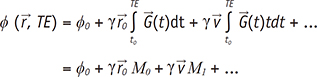
Here, the first term on the right-hand side (ϕ0) is the background phase offset which is influenced by the field inhomogeneity. The second and third are the phase accumulations from the stationary and moving spins, respectively, under the magnetic gradient . The integral terms describing the influence of the magnetic gradient on the static and moving spins are named the zeroth and the first gradient moments, M0 and M1, respectively.
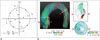
. The integral terms describing the influence of the magnetic gradient on the static and moving spins are named the zeroth and the first gradient moments, M0 and M1, respectively.Conventional 2D PC-MRI uses a bipolar gradient along the flow-encoding direction before the readout sequence (Fig. 1). The bipolar gradient removes the phase accumulations from the stationary spins, which results in only the background phase offset and the flow-related phase accumulations (the first and third terms in Eq. 2). The PC-MRI sequence typically uses two acquisitions with different M1 values to remove the unknown phase offset. In 2D PC-MRI, two acquisition schemes are conventionally used. The first type of the acquisition scheme employs the flow-compensation gradient with the flow-encoding gradient to obtain the reference image. The second type of the acquisition employs the combination of the flowencoding gradient and the following gradient with the opposite polarity. Meanwhile, the no bipolar gradient for the reference image is rarely used. In 4D PC-MRI, the first acquisition scheme is mostly used, and the reference acquisition without the bipolar gradient is rarely used.
The phase difference between the two scans is directly related to the velocity of the flow as follows:

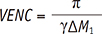
The velocity-encoding parameter, which is named Venc or VENC, determines the maximum velocity by changing the difference in the first gradient momentum ΔM1 as follows:
Here, it can be noted that the flow velocity that is as high as the pre-determined VENC (cm/s) gives the phase shift of π.

In contrast to conventional 2D PC-MRI with two acquisitions, 4D PC-MRI usually uses four-point scans by measuring the three-directional velocity encodings and one-flow compensation encoding, as shown in Figure 1 (26). Assuming the background phase offset is the same in the four different scans, the three-directional velocities can be obtained by substituting the phase shifts in the three-directional encodings with the phase in the reference image.
4D PC-MRI usually exports three-directional volumetric phase images for velocity reconstruction, one volumetric magnitude image, and four volumetric vector difference images (three-directional images and one summation image) for depicting vascular anatomic information (2728). The exported images vary according to the vendor and sequence of the MRI scanner.
Image Acquisition and Analysis Procedures
Scan Parameters
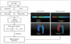
When a patient is registered for 4D PC-MRI, adequate scan parameters need to be used to obtain data of sufficient quality with a reasonable scan time. Of the various scan parameters, the most important parameters include field of view, spatial resolution, temporal resolution, and the VENC (Fig. 2). The field of view would ideally encompass the entire vasculature, but a larger field of view requires a greater amount of scan data and, consequently, a longer scan time. Therefore, the field of view should be confined to the smallest region that contains the region of interest, in order to reduce the scan time.
The spatial resolution should also be as high as possible because a higher spatial resolution results in more accurate flow quantification and helps to identify smaller-scaled flow phenomena (29). However, the smaller the voxel, the longer the scan time and the lower the signal-to-noise ratio (SNR). Therefore, a compromise between the spatial resolution, scan time, and SNR is needed for scanning. Practically, voxel sizes of 2.5–3.0 mm and 0.7–1.5 mm are usually used to measure cardiac blood flow and intracranial blood flow, respectively (303132333435).
Temporal resolution should also be as short as possible to accurately identify temporal variations in pulsating blood flow. However, in 4D PC-MRI, the number of MRI signal acquisitions is directly proportional to the number of cardiac phases, which is the number of temporal steps of the data for describing the whole pulsatile cycle. Therefore, the temporal resolution is limited to reduce the total scan time. Typically, a temporal resolution of around 40 ms is usually used to measure pulsatile aorta flow (3135).
As described in Imaging Principles section, the VENC determines the maximum encoding velocity of the blood flow. Because a flow velocity higher than the pre-determined VENC will result in phase aliasing, the VENC should be higher than the expected maximum velocity of the flow. However, because a higher VENC will also decrease the velocity-to-noise ratio, a VENC around 10% higher than the expected maximum velocity flow is usually recommended (30).
In addition to the parameters described above, various other parameters, including partial k-space coverage, parallel imaging, and k-t undersampling, also need to be considered to limit the scan time and improve the SNR of the data. For a more detailed description of the scan parameters, readers should refer to previous reviews of 4D PC-MRI (1030).
Pre-Processing
Even though 4D PC-MRI scanning exports various types of reconstructed images, as described in Imaging Principles section, the phase image from the 4D PC-MRI is preferred for further processing, such as flow quantification and analysis. However, the phase image includes various types of inherent errors. Therefore, pre-processing of the raw data is required.
The phase image from the PC-MRI sequence has phase offset errors from the concomitant gradient (or Maxwell terms) (36), gradient field non-linearity (37), and eddy currents (38). The existence of these background phase errors should be understood, and the corresponding correction schemes are required for phase correction. Commercial analysis software for 4D PC-MRI, such as 4D Flow (Siemens, Munich, Germany), GT-Flow (Gyrotools LLC, Winterthur, Switzerland), CAAS MR 4D Flow (Pie Medical Imaging BV, AJ Maastricht, the Netherlands), and Arterys (Arterys, San Francisco, CA, USA), provides phase correction schemes. However, to adjust the correction schemes to their own data, most researchers continue to use their own correction schemes based on MATLAB (Natick, MA, USA) or other programming languages.
If the flow velocity is higher than the pre-determined VENC, the raw data will contain phase aliasing or phase wrapping. If the flow quantification is processed without considering the phase aliasing, the results will be severely corrupted by the phase aliasing. Therefore, if such phase aliasing is unavoidable, a phase-unwrapping algorithm is needed to recover the information from regions of phase aliasing. However, a generalized algorithm for phase unwrapping has not been derived yet, and each algorithm may have different performances according to the characteristics of the phase data. Therefore, several studies have been performed to determine phase-unwrapping algorithms and compare the performances of various algorithms (394041424344).
Once the raw data have been appropriately corrected, the next step is image segmentation to generate masking images to distinguish the fluid region and the external static tissues in the phase images. Because the sum of vector difference image (Fig. 1), named the complex difference image, can clearly distinguish the flow and the surrounding region, this image is usually used as an angiogram for identifying arteries and veins from the static surrounding tissues (2728). If the sum of vector difference image does not have enough contrast between the fluid and static tissues due to a slow flow, a separate 3D MR angiography scan can also be used for registration. To generate the mask images from the angiograms, various types of segmentation schemes can be used, from manual segmentation based on pre-knowledge of the anatomy of interest to fully automatic mask generation (454647).
Data Analysis
To analyze and visualize hemodynamic features using 4D PC-MRI, two approaches are available. The first option is to use commercial analysis tools for 4D PC-MRI. The commercial tools described in Pre-Processing section can be easily used to visualize and quantify the results. However, the commercial tools still provide only a limited number of basic flow parameters such as flow rates and volumes. Accordingly, most researchers calculate their own parameters based on their own platforms using MATLAB or other programming languages, and then visualize and analyze their data using conventional post-processing tools that are popular in the field of fluid dynamics, such as Tecplot (Tecplot, Bellevue, WA, USA) and Ensight (CEI, Apex, NC, USA).
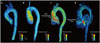
The visualization of 4D PC-MRI data usually uses vector field, streamline and pathline (Figs. 3, 4, 5, 6, 7, 8). A velocity vector field is a collection of velocity vectors in space (Fig. 3). It visualizes the speed and direction of the blood flow with a collection of arrows with a given magnitude and direction. Streamline is defined as a collection of curves that are tangent to the velocity vector of the flow at the specified time (Fig. 3). It resultantly indicates the direction of fluid element at the specified time point. On the other hand, the pathline is a collection of the trajectories that an individual fluid element flows over a certain time (Fig. 8). As a result, it indicates how each fluid element moves during the cardiac cycle.
Hemodynamic Quantification
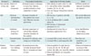
While 4D PC-MRI provides the same basic flow quantifications as conventional 2D PC-MRI, the multidimensional data of 4D PC-MRI has facilitated the development of various fluid dynamic biomarkers for better assessing blood flow in vivo. The following sections introduce the principles and physiological meanings of the hemodynamic parameters that can be obtained using 4D PC-MRI (Table 1). However, most commercial software does not cover all of these quantifications. Therefore, the development of in-house software is required for these quantifications.
Velocity and Flow Rate
The velocity and flow rate of blood flow are the most basic fluid dynamic parameters used to compare the normal and pathological conditions of blood flow against baseline. A decreased local flow rate directly indicates the loss of blood being transported toward the corresponding tissue regions, which could be the result of local ischemia (48). A local increase in the blood velocity at stenotic regions, such as regions with aortic valve stenosis or aortic coarctation, is related to the severity of the stenosis (4950). Because 4D PC-MRI provides whole velocity data within the volume of interest, it is useful for quantifying the flow rate distribution of complex vessel networks and estimating the peak velocity within certain regions.
The velocity of the blood flow calculated from the 4D PC-MRI data is usually visualized using pathlines and streamlines with velocity color mapping (Fig. 3). For any arbitrary cross-sectional plane within the volumetric data, retrospective quantification of the flow rate can be carried out by integrating the velocity inside the specified lumen. Previous studies found that the velocity and flow rate from 4D PC-MRI were well correlated with those from 2D PC-MRI (51). Practically, around three voxels along the vessel diameter (around five voxels across the lumen area) were sufficient to accurately quantify the flow rate (29). However, the accuracy of the flow rate quantification using 4D PC-MRI can be at least somewhat influenced by the segmentation of the vessel because 4D PC-MRI generally has lower spatial resolution than 2D PC-MRI. Therefore, the accurate segmentation of the geometrical boundary of the vessel is important when assessing flow rate on 4D PC-MRI.
Wall Shear Stress
Wall shear stress is the frictional shearing stress exerted by fluid on the vascular wall. Recently, WSS distribution in arterial blood flow has received considerable attention because it has been associated with vascular diseases, specifically, atherosclerosis and aortic dilatation (234). By definition, WSS can be obtained by multiplying the viscosity of the fluid by the local velocity gradient at the wall as follows: where τ is the WSS, n is the local wall normal displacement vector, u is the local velocity component, and µ is the dynamic viscosity. The unit of WSS is Pa or N/m2 when the units of u, n, and µ are m/s, m, and N·s/m2, respectively.

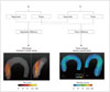
The first step for WSS estimation is to obtain a smooth spline contour or surface of the lumen from the magnitude, phase, or mask images, so that the wall location and normal displacement vector can be estimated from the lumen contour or surface (Fig. 4). Then, the velocity near the wall along the normal vector is obtained by interpolating the neighboring velocity data, and the velocity gradient at the wall is calculated on the vessel lumen using the spline interpolation model, which provides the analytical derivative of the flow velocity (52). Consequently, WSS can be obtained by multiplying the obtained velocity gradient by the blood viscosity by assuming that the blood viscosity is constant at around 4 centipoise (cP) (52). Finally, the obtained WSS is usually visualized using color-mapped surface rendering to distinguish the low and high WSS regions, and is quantified with segmentation (Fig. 4).
Turbulent Kinetic Energy
While the blood flow mostly comprises laminar flow, under certain conditions blood flow can be turbulent with high-velocity fluctuations. In particular, arterial blood flows with local contractions due to aortic valves, aortic coarctation, and atherosclerosis, usually develop a local turbulent blood flow (1718). Quantification of the turbulent velocity fluctuation is important because it increases the pressure drop along the vessel by elevating the fluid energy dissipation, which consequently results in a requirement for more energy to maintain the perfusion of the blood flow (53). In addition, a higher turbulence of the flow than baseline under similar flow rate conditions also indicates more severe stenosis (17).
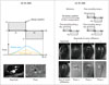
Previously, Dyverfeldt et al. (16) derived an equation for TKE estimation based on the relationship between the intravoxel velocity distribution and the MR signal from a standard PC-MRI scan (Fig. 5). This estimation assumes that the spin velocities within a voxel are normally distributed in turbulent flow. Three-directional standard deviation components of the turbulent flow can be obtained from the magnitude images of the four-point scans as follows (54): where σi indicates the standard deviation in the ith-direction (x, y, z), kv indicates the net motion sensitivity (kv = π / VENC), and |S0| and |Si| indicate the magnitude of the MRI signal obtained without and with flow sensitivity, respectively. The TKE per unit volume can be estimated from σ as follows: where ρ is the fluid density and σi indicates the standard deviation in the ith-direction (x, y, z).

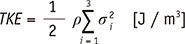
Importantly, the sensitivity of TKE estimation is influenced by the VENC (or kv). The sensitivity of the TKE estimation is optimal when the signal magnitude ratio |S|/|S0| becomes approximately 0.6 (analytically: e-1/2) (16). However, the VENC value for obtaining |S|/|S0|–0.6 is usually less than the maximum velocity of the flow; consequently, the scan for TKE estimation usually results in phase aliasing. Therefore, at least two acquisitions with different VENC values are generally requested to obtain both the velocity field and TKE distribution.
Vortical Structure
Blood flow frequently generates vortical flow patterns (e.g., locally rotational or helical flows) in various cardiovascular regions, including the left ventricle, ascending aorta, and pulmonary vessel (555657). While the in-depth relationship between the vortical flow and the pathology is not yet fully understood, the existence and intensity of the vortical flow are influenced by pathological conditions, such as aortic aneurysm, pulmonary hypertension, and heart disease (555657). Therefore, accurate quantification of the vortical flow structure is important in revealing the relationship between vortical flow structures and vascular diseases, and to develop a fluid dynamic index based on the vortical flow structure.
Vorticity
One of the basic fluid dynamic parameters describing the rotational motion of the fluid element is the vorticity vector of the flow. Vorticity  is defined as the curl of the velocity vector : where ∇ is the del operator. Here, each vorticity component indicates the swirling intensity of the fluid element along the corresponding axis (Fig. 6A). The unit of vorticity is s-1.
is defined as the curl of the velocity vector : where ∇ is the del operator. Here, each vorticity component indicates the swirling intensity of the fluid element along the corresponding axis (Fig. 6A). The unit of vorticity is s-1.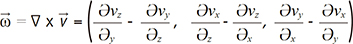
λ2-Criterion
The λ2-criterion is the one of the most popular methods for identifying the vortical flow structure (58). This algorithm is based on the velocity gradient tensor J, where  . Then, the velocity gradient tensor can be decomposed into the symmetric S and asymmetric Ω terms as follows: where T indicates the transpose of the matrix. Identification of the eigenvalues of S2 + Ω2 for each voxel results in three eigenvalues, λ1, λ2, and λ3, where λ1 ≥ λ2 ≥ λ3. Finally, the vortex flow region can be found where λ2 is negative. Since this algorithm is Galilean invariant, the vortical flow structures can be identified even though the vortical flow is overlaid with the uniform translational velocity field.
. Then, the velocity gradient tensor can be decomposed into the symmetric S and asymmetric Ω terms as follows: where T indicates the transpose of the matrix. Identification of the eigenvalues of S2 + Ω2 for each voxel results in three eigenvalues, λ1, λ2, and λ3, where λ1 ≥ λ2 ≥ λ3. Finally, the vortex flow region can be found where λ2 is negative. Since this algorithm is Galilean invariant, the vortical flow structures can be identified even though the vortical flow is overlaid with the uniform translational velocity field.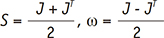
Critical Point Analysis
Critical point analysis is also a vortex structure identification method based on critical point analysis of the local velocity gradient tensor and its corresponding eigenvalues (5960). The eigenvalues of the local velocity gradient tensor J have one real eigenvalue (λr) and a pair of complex conjugate eigenvalues (λcr ± iλci) when the discriminant of its characteristic equation is positive. Then, λci -1 represents the period required for a fluid particle to rotate along the λcr axis (61). Therefore, the region with nonzero λci corresponds to the local vortical flow, and the magnitude of λci is related to the intensity of the vortical flow. This method is also Galilean invariant and contains information on the strength of the vortical flow, in contrast to the λ2-criterion (Fig. 6B).
Non-Invasive Estimation of Pressure Drop
A blood flow pressure loss indicates the loss of flow energy generated from the heart. An increase in the energy loss results in decreased blood flow or an increased workload on the heart for maintaining the same flow rate. Therefore, the pressure gradient is widely used as an important biomarker of stenosis severity, such as that caused by aortic valve stenosis or aortic coarctation (6263).
Application of a pressure catheter has been a gold standard method for measuring the pressure values in vivo. However, it is not preferred due to its invasiveness. Alternatively, the pressure gradient can be estimated by Doppler echocardiography, which is a non-invasive method for measuring the maximum velocity of the flow across the stenosis region and estimating the pressure gradient based on a simplified Bernoulli equation (64). However, this method does not provide the spatial and temporal variations in the pressure. In addition, the accuracy of the results can vary according to the flow conditions because the simplified Bernoulli equation assumes the flow is laminar without turbulence, and it also neglects the viscous energy dissipation (65).
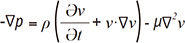
Recently, relative pressure estimation using 4D PC-MRI has been introduced as an alternative method for estimating the pressure loss of the blood flow across the aorta and stenosis (236566). The method aims to calculate the pressure gradient at each voxel from the Navier-Stokes equation and reconstruct the pressure field over the entire vessel of interest (Fig. 7). Assuming that blood is a viscous, incompressible fluid, the Navier-Stokes equation can be arranged as follows: where p is the pressure, µ is the viscosity, ρ is the density, and v is the velocity. Here, the gravitational term has been neglected. Because the temporal variations in the 3D velocity can be obtained from 4D PC-MRI, the spatial gradient of the pressure can be easily obtained using Eq. (11). Once the pressure gradients over the volumetric regions are obtained, the spatial and temporal variations in the relative pressure field can be obtained by solving the Poisson pressure equation. Notably, the pressure field obtained from Eq. (11) is a relative pressure field without the absolute pressure reference. Therefore, only a pressure gradient can be estimated from the present method without any reference pressure, and the absolute pressure value cannot be obtained.
Clinical Applications
While 3D volumetric acquisition of blood flow using 4D PC-MRI takes a long time compared with conventional 2D PC-MRI, it has its own advantages by permitting retrospective investigation of the blood flow for any arbitrary cross-sectional plane within the volumetric data. For this reason, 4D PC-MRI can be useful when multisectional scans of 2D PC-MRI are needed. Previous studies showed that 4D PC-MRI was effective for quantifying the flow rates through various cardiovascular and intracranial arteries and veins with single volumetric acquisition, and the quantification results were comparable with those of conventional 2D PC-MRI (325167).
While quantifications of the shunt flow or regurgitation flow using 2D PC-MRI can be inaccurate because the valvular regions move inherently during the cardiac cycle, 4D PC-MRI can consider the motion of the regions of interest. Therefore, 4D PC-MRI can be routinely used as a clinical tool for measuring inlet and outlet valve flow as well as the regurgitation flow through the cardiac valve (1468).
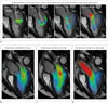
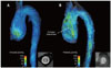
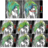
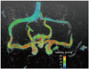
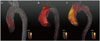
In addition, visualization of the time-resolved 3D flow field using 4D PC-MRI enables characterization of the vascular disease-related alteration of blood flow structures by reference to the baseline flow characteristics. Previous studies reported that complex blood flow can be intuitively visualized by describing the transit and accumulation of the blood and the vortical structure identification, and these visualizations were effective for diagnosing the dysfunction of the left ventricles (Fig. 8) (566970), the aortic valves (Figs. 9, 10) (4, 71), pulmonary hypertension (Fig. 11) (57), and intracranial blood flow (Fig. 12) (72, 73).
Recently, some multidisciplinary researchers have developed various hemodynamic parameters based on fluid dynamics and demonstrated their clinical implications. WSS is one of the most popular indices for assessing blood flow abnormalities. Recent studies using 4D PC-MRI found that regions of high WSS correspond with extracellular matrix dysregulation and elastic fiber degeneration in the ascending aorta (74). Thus, abnormal WSS might play a major role in the development of aortopathy. Consequently, WSS quantification using 4D PC-MRI could be an important biomarker of disease progression (3474). In addition, WSS is suspected to be associated with intracranial aneurysm rupture (75). Therefore, various studies have investigated the feasibility of WSS quantification to predict the risk of intracranial aneurysm (7677).
Quantification of TKE using 4D PC-MRI is also a promising biomarker of the efficiency of the blood flow. One study assessed the in vivo feasibility of the use of TKE quantification to detect cardiovascular flow abnormalities such as those caused by aortic valve flow and aortic coarctation (18). Recent clinical studies found that patients with dilated cardiomyopathy had higher TKE than healthy subjects (78). In addition, TKE quantification was used as a non-invasive tool for quantifying the severity of aortic stenosis because the TKE value in the ascending aorta was strongly correlated to index pressure loss (Fig. 13) (17).
Non-invasive quantification of the relative pressure using 4D PC-MRI has been mostly developed and validated using aortic flow because the larger vessel guarantees more suitable results (2365667980). Although 4D PC-MRI does not provide the absolute pressure value, it still provides the pressure drop information across the aortic coarctation and its temporal variations, such that a time-resolved pressure gradient can be used to assess disease severity (Fig. 13) (65). Non-invasive pressure distributions have also been used to assess carotid, iliac, and renal arteries with stenosis (8182). In addition, the pressure field in various types of intra-aneurysms was also validated with invasive microcatheter pressure validation (83). Compared with the point-wise measurement of the catheter-based pressure approach, non-invasive pressure estimation using 4D PC-MRI provides a time-resolved 3D relative pressure field, so that it can identify the relationship between the fluid pattern and the spatial distribution of the dynamic pressure. Consequently, regions with a local peak pressure and spatial deviations could be easily assessed, which cannot be done with invasive catheter pressure measurement (83).
In addition to the previous quantifications, 4D PC-MRI can also be used to measure pulse wave velocity to assess arterial stiffness and evaluate atherosclerosis progression (2484). Pulse wave velocity estimation using 4D PC-MRI acquires volumetric velocity data in the entire aorta and estimates the temporal lag of the blood pulse between the ascending and descending aortas. This parameter was well correlated with the conventional pressure catheter-based estimation and clearly distinguished patients with atherosclerosis from normal controls (2484).
While the present article focused on describing quantitative hemodynamic parameters using 4D PC-MRI, it can be noted that many clinical research studies using 4D PC-MRI have also found the utility of qualitative or semi-quantitative analysis of abnormal blood (8586). Compared to the normal subjects, the patients with bicuspid aortic valve and aortic stenosis showed frequent helical flow patterns in the ascending aorta (486). In addition, the eccentricity of the aortic flow was also a reliable method for determining the abnormality of the aortic flow (85).
Limitations and Potential
A long scan time is the one of the main limitations of 4D PC-MRI when measuring volumetric regions. Measurement of the major vessels in the head, thorax, and abdomen with a conventional 4D PC-MRI sequence with Cartesian k-space filling takes around 20 minutes when the practical levels of the scan parameters are used (10). The scan time can vary depending on various scan parameters, such as field of view, spatial resolution, temporal resolution, and parallel imaging. Adjusting these parameters to reduce the scan time generally reduces the SNR of the data, which strongly influences the accuracy of the quantifications. Therefore, an appropriate compromise between the scan time and the SNR should be made by considering the objectives of the study. Recently, various new sequences for accelerating the acquisition have been developed, such as k-t undersampling (87), radial sampling (88), and stack-of-stars (89).However, these advanced schemes require further validation before they can be considered suitable for clinical use.
Based on the principle of PC-MRI, each voxel provides the spatially and temporally averaged value of the signal within the voxel (90). Complex blood flow, such as turbulent flow, has a wide range of flow scales, from a few micrometers to a few centimeters, and the temporal spectrum ranges from a few microseconds to a few seconds. Therefore, clinicians and researchers should note that 4D PC-MRI is unable to resolve all blood flow structures, and they need to optimize the spatial and temporal resolutions of 4D PC-MRI by considering the spatiotemporal scales of the flow features of interest.
Although 4D PC-MRI can provide new information to physicians that cannot be found with other imaging modalities, there is no suitable guideline for the use of 4D PC-MRI. A previous guideline for cardiac magnetic resonance could be a useful basis for the future guideline for 4D PC-MRI (91).
The noise of 4D PC-MRI is also one of its limitations. Because the VENC determines the noise level of the velocity field, low-velocity regions are usually less reliable than high-velocity regions due to the overlaid noise. While hemodynamic parameters based on the integration of the velocity field, such as flow rate, are less sensitive to this noise, other estimated parameters based on the derivatives of the velocity field can be significantly influenced by the noise level. Therefore, the influence of the background noise on the quantification of the resultant parameters should be assessed to guarantee the veracity of the results.
For more accurate quantification, pre- or post-processing is vital. Most of these problems depend on the difficulty of image segmentation due to poor image contrast, which could be improved by registration with a separate MR scan, such as balanced steady-state free precession (92) and/or CT angiograms. However, so far, little in-house software has been developed to carry out the segmentation and quantification of 4D flow MRI.
CONCLUSION
Four-dimensional PC-MRI has been improved by the rapid development of sequence, reconstruction, and post-processing techniques. Multidirectional velocity flow measurement with volumetric acquisition enables various retrospective analyses, which might be useful in clinical practice. Multidisciplinary researchers have developed several potential biomarkers based on fluid dynamics, and these biomarkers are being validated in various clinical investigations. While 4D PC-MRI is still being used only for research purposes, it will no doubt soon be available for routine clinical applications as the clinical evidence accumulates.


 XML Download