

 PDF
PDF ePub
ePub Citation
 Print
Print


INTRODUCTION
In dentistry and orthodontics, image data plays a key role in the analysis of treatment outcomes. Traditionally, cephalometric measurements taken from radiographs have served as key indicators when studying shape and size change over time, or shape and size differences between patients or treatments. Cephalometric landmarks are well-defined in the literature, and distances or angles between landmarks are often used to describe clinical features for statistical analysis. In recent years, three-dimensional (3D) imaging modalities have become more readily available, and present a number of advantages. Methods such as cone-beam computerized tomography (CBCT) have relatively low radiation dosages, and present a clear view of bony structures with minimal image distortion (1-7). Additionally, structures or landmarks not easily available on traditional two-dimensional (2D) imaging (such as dental pulp chambers) may now be identified (8).
Traditionally, when landmark data is used for statistical analysis in dentistry and orthodontics, specific inter-landmark distances or angles are chosen. This method works well in cases where only a small number of specific lengths or angles are of clinical interest, or when there is a very specific outcome desired. In this paper, all landmarks for a given subject are taken together as one configuration, and analyzed using tools from the relatively new area of computational mathematics called persistent homology (9, 10). The goal of this method of analysis is to compare overall effects of treatment across different groups and time points, without having to specify a small number of measurements for individual analysis.
In this study, our new method is applied to a data set which compares bone- and tooth-anchored rapid maxillary expansion (RME) treatments to a control group over time. Maxillary transverse deficiency is a common problem in orthodontic patients, and is traditionally corrected by RME using a tooth-anchored expander (Hyrax). However, tooth-anchored appliances present undesirable tooth movement (11), root resorption (12), and lack of firm anchorage to retain sutural long-term expansion (13). In addition, there is evidence that tooth-borne forces produce only limited skeletal movement (14). An alternative to tooth-anchored expansion is to employ a bone-anchored method anchored directly to the palatal surfaces of the maxilla. This method is more invasive and this is a disadvantage (along with a higher risk of infection) (15, 16). This has been reported by Lagravère et al. (8) where results using traditional methods of statistical analysis show no significant difference between appliances. Thus, the purpose of this paper is to describe a method for the statistical analysis of 3D landmark configuration data, and apply it to the orthodontic clinical trial data set comparing two types of RME treatment with a control group (8).
MATERIALS AND METHODS
The method we present consists of two main parts. The first is persistent homology, which takes a set of points and gives information about various features of interest (as discussed in the section 'Method for comparing landmark configurations'). The second step is a dimensionality reduction method which takes the rich information output from persistent homology, and represents it in a low number of dimensions, suitable for further statistical analysis.
Orthodontic Data Set
The dataset discussed in this paper was obtained from a study at the University of Alberta Orthodontic Graduate Clinic involving two types of maxillary expanders. Sixty-two patients from the clinic's patient pool were recruited during an 18 months period and all of these patients were diagnosed as requiring maxillary expansion treatment. They were randomly allocated into one of three groups: bone-anchored maxillary expansion treatment, tooth-anchored maxillary expansion treatment, and a control group, with treatment delayed for 12 months during the study period. The bone-anchored maxillary expansion system consisted of two stainless steel onplants, two miniscrews, and an expansion screw, with each onplant secured directly to the palatal bone surface with the miniscrews. The tooth-anchored maxillary expansion treatment was performed using the traditional Hyrax with bands on the first permanent molars and first premolars. Appliances were activated until overcorrection was achieved, and then left passively in place until six months had elapsed since appliance insertion. Full details of the activation methods and descriptions of expander insertion techniques are given in Lagravère et al. (8).
Three-dimensional images were taken of each patient using CBCT (Newtom 3G, Aperio Services, Verona, Italy) at four time points: at baseline (time 1), after completion of activation of the appliance (time 2, approximately 2 weeks for tooth-anchored and 2 months for bone-anchored), after removal of the appliance (time 3, 6 months), and prior to fixed bonding (time 4, 12 months). To minimize radiation exposure, the control group only received CBCT scans at baseline, 6 months and 12 months, so it was assumed that no change had occurred between time points 1 and 2, and time point 1 data was used at both time points 1 and 2.
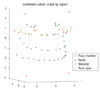
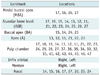
To perform the subsequent analysis, the scan of each patient at each time point was used to obtain a configuration of sixty-eight landmarks, which served as a geometric representation of the maxillary complex. The landmarks that were used are described in Table 1, and their mathematical representation is shown in Figure 1. The landmarks were placed on each image by experienced practitioners, with landmark placement checked for reliability (mean measurement differences were less than 0.7 mm along each axis for each landmark). Three subjects did not have the entire set of landmarks available due to missing teeth, and were excluded from the analysis presented in this paper. Therefore, for our purposes a total of 59 subjects were used, with 20 in each of the treatment groups and 19 in the control group. Across the four time points, this gave a total of 236 configurations (with each subject at each time point represented by one landmark configuration).
Method for Comparing Landmark Configurations
To begin this section a question arises: in order to perform statistical comparisons, how do you define the distance between two landmark configurations? This question is addressed in the field of statistical shape analysis. Those methods often produce good results, but face difficulty with large between-subject variability in the data. The method that we discuss in this paper is one presented in Gamble and Heo (17). As mentioned in the introduction, it involves the use of a method from computational mathematics called persistent homology, combined with methods of dimensionality reduction, to obtain a few types of distances measures between landmark configurations. As far as we are aware, this is the first time that persistent homology is applied to 3D data in an orthodontics study. Thus, we provide a brief explanation of the technique.
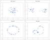
Persistent homology (9, 10) is a mathematical method which quantifies information about the structure of a set of data points. The types of data features that this method quantifies are features that mathematicians call 'topological features', which include the number of separate components, number of holes, or the number of voids. These features are said to be of dimension zero, one and two, respectively. For example, the number of separate components is a zero-dimensional feature, and a set of points which are grouped into two clusters would be considered 'different' than a set of points that are all grouped closely together. These clusters are similar to the groupings obtained through the statistical method of cluster analysis. When considering one-dimensional features, a set of points that formed a small loop would be different from points in a random cloud, but would also be different from points that form a large loop (or even two or more loops). Similarly, enclosed voids (like the inside of a soccer ball) are 2D features of interest. Quantification of features such as these can help to distinguish the subjects whose features vary in number or size. Examples of zero- and one-dimensional features that are different in number are given in Figure 2. The zero-, one- and 2D features for the current data set are mentioned in the Results section, and detailed in the Discussion section.
Persistent homology takes information about the number and size of these topological features, and quantifies them for each dimension. Not only can this method describe the features for a given set of data points, but a distance has been defined in the persistent homology literature to compare how similar two sets of data points are with respect to their topological features. In mathematics, the number of i-dimensional features (i.e. the number of components, loops or voids for i = 0, 1 and 2) is denoted by βi, so we will call the distance between two point sets with respect to their zero-dimensional features the 'β0 distance', and the distance with respect to their one- and two-dimensional features as the β1 and β2 distances.
The representations of the topological features that persistent homology quantifies are relatively complicated structures, that do not exist in Euclidean space (like values on the real line do), but the distances between them can still be calculated in a pairwise fashion. For a number of point sets (say n) under analysis, the distances between all the pairings are recorded in a n-by-n matrix. Thus, for the 236 landmark configurations under comparison in our analysis, the β0, β1, and β2 distances between them were each represented in a 236-by-236 matrix. To allow traditional statistical analyses to be employed, dimensionality reduction was used on each n-by-n matrix to obtain a lower dimensional embedding of the n points which preserved the distances between them as efficiently as possible. The most information about the variability was in the first embedded coordinate, with successively less information added with each additional coordinate, so only a small number of the embedded coordinates were chosen for analysis. For our analysis, we used the non-linear method of dimensionality reduction called Isomap (18).
For each of the β0, β1 and β2 distance matrices obtained from persistent homology, a lower dimensional embedding is obtained, consisting of a few coordinate dimensions. The first coordinate obtained from the βi distances is called the first βi embedded coordinate, and it represents the greatest variability in i-dimensional features in the landmark configurations.
In order to interpret the embedded coordinates, the correlations were calculated between the embedded coordinates and each of the inter-landmark distances. The regions were then identified that correlate most strongly to each embedded coordinate. Additionally, the mean shapes (19) were obtained using subjects with small, middle, or large coordinate values, and compared to see if any obvious shape differences were visible. A plot of representative embedded coordinates is shown in Figure 3, with the lowest, middle and highest 10% of coordinate values colour coded. The first β0, β1 and β2 embedded coordinates were each analyzed using repeated measures ANOVA to determine whether differences were identified between the treatment groups over time. When reporting results of the statistical analyses, a p-value below 0.05 was considered significant. However, 'weakly significant' p-values between 0.05 and 0.1 are also reported here to illustrate trends in the data that do not reach the standard cut off for significance. The computer code used for the computations in this paper was adapted from the program PLEX (20), and run in MATLAB (MATLAB R2008a, MathWorks, Natick, MA, USA).
RESULTS
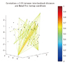
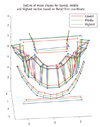
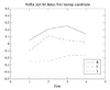
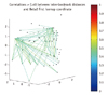
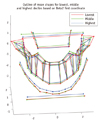
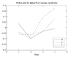
The first β0 coordinate represents the size and number of zero-dimensional topological features (i.e. the size and number of separate components). Since all the configurations consist of one component (the craniofacial complex), this coordinate is mainly associated with size, and with inter-landmark distances that are far apart. Figure 4 shows the inter-landmark distances that are most strongly correlated (r > 0.55) with the first β0 coordinate run diagonally and vertically between the infra orbital and menton landmarks, and between the menton and maxillary landmarks. It seems that this coordinate is an overall size measure, but is particularly related to vertical length. This is confirmed in Figure 5 which shows the outline of the mean shape obtained from the landmark configurations with the 10% lowest, middle, and highest first β0 coordinate values. It can be seen that the largest coordinate values correspond to relatively higher infra orbital landmarks, and lower menton landmarks, indicating a vertical elongation compared to the other subjects. To see if there are any significant differences between the treatment groups or over time with respect to this coordinate, a repeated measures ANOVA was performed using the factors time and group, as well as the time*group interaction. Overall, this coordinate shows significant changes over time (p = 0.001 approx.), and how the change occurs is not the same for all groups (interaction significant, p = 0.024). In this coordinate, differences were most pronounced at Time 2, when the bone-anchored group was significantly different from the control group (p = 0.033), and the difference between the control and tooth-anchored groups was weakly significant (p = 0.077). No significant differences between groups were seen at time points 3 and 4, although looking at the profile plot (Fig. 6), the mean values for the two treatment groups seem to be higher than for the control group.
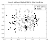
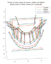
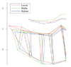
The first β1 coordinate conveys information about one-dimensional topological structures. For this data set, it is most strongly related to inter-landmark distances that cross the maxilla, both horizontally and diagonally, as well as inter-landmark distances that run diagonally between the menton and infra orbital landmarks and the maxilla (Fig. 7). This is visualized in Figure 8, showing the outlines for the mean shapes based on the lowest, middle, and highest 10% of first β1 coordinate values. The mean based on the lowest coordinate values (shown in red) is considerably smaller both vertically and in width. It appears that this coordinate is also an overall size measure (similar to β0), but with more emphasis on maxillary width (in addition to vertical height). If this measure does indeed correspond to maxillary width, then statistical analysis should be able to discern treatment effects (i.e. an increase in coordinate values) in the two maxillary expansion groups over time. Repeated measures ANOVA in fact shows significant overall time effects (p = 0.001 approx.), with the profile plot (Fig. 9) showing a slight increasing trend over time for the control group, and a strong increase in the treatment groups from Time 1 to Time 2. The treatment groups relapse slightly towards Time 4. When comparing the groups at individual time points, the bone and control groups are significantly different from each other at both Time 2 (p = 0.014) and Time 3 (p = 0.038), whereas the tooth-anchored group is only slightly different from the control at Time 2 (p = 0.069), and not significantly different at the other time points.
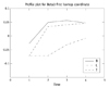
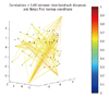
One of the most interesting results was in the first β2 coordinate, where the analysis uncovered something that the researchers were not looking for. When looking at the inter-landmark distances that had strongest correlation with the first β2 coordinate (Fig. 10), and the plots of the mean shapes for the lowest, middle and highest 10% of coordinate values (Fig. 11), the landmarks most heavily involved were all related to the first and (especially) second molars. When looking specifically at the second molar region on the outline plot (Fig. 12), it can be seen that the subjects with lowest coordinate values had substantially higher root apex and pulp chamber landmarks in the second maxillary molars. Since the alveolar bone landmark is defined as being directly lateral to the root apex, the bone pertaining to this specific area is farther from the root apex compared to other teeth, resulting in the set of second molar landmarks appearing to have a much larger configuration. This type of configuration corresponds to unerupted second molars. Subjects with larger embedded coordinate values tend to have second molars that are more fully erupted (with lower root apex and pulp chamber landmarks, and alveolar bone landmarks much closer to the root apex). This coordinate displays variability between the subjects in degree of second molar eruption, but to determine whether there were any differences between the groups or over time, a repeated measures ANOVA was performed using the first β2 coordinate. Overall, time was seen to be significant (p = 0.015), but there were no significant differences between groups at any of the time points, and no time*group interaction was found. A profile plot of the first β2 coordinate for the three groups over time is shown in Figure 13. The general increasing trend over time, along with no obvious differences between the control and treatment groups, indicates that the changes seen were due to natural tooth eruption and not treatment effects.
DISCUSSION
In this paper we have discussed a method for the analysis of landmark-based data, which considers entire configurations at once, and determines distances between configurations based on topological features of various dimensions. The method was applied to an orthodontic data set from a study of two rapid maxillary expansion treatments and a control group over time, and the method was able to determine a number of significant features in the data. The most predominant feature was maxillary width, which was found to increase significantly from Time 1 to Time 2 in the treatment groups, with a slight regression at later time points. Significant differences in the coordinate corresponding to maxillary width were seen between the bone-anchored and control groups at Time 2 and Time 3. The fact that the first β1 coordinate had strongest associations with maxillary width, and displayed the treatment effects most prominently is likely due to the fact that the β1 coordinate displays variability in one-dimensional features of the data, and the maxilla is essentially a 'U-shaped' structure (which is topologically one-dimensional).
The first β0 coordinate expressed overall size, particularly a vertical component of size, which varied both over time and between groups. The trend seen over time was an increasing one, with the control group increasing slowly over time, and the treatment groups increasing more dramatically from Time 1 to Time 2, and then gradually afterward. The vertical elongation that was seen in the treatment groups could possibly be due the slight opening of the mouth due to the initial expansion and relocation of the teeth involved in the expansion area changing the occlusal pattern temporarily, which is often noted clinically.
An unexpected result of the analysis was shown in the β2 first coordinate, which was able to distinguish variability in the subjects related to degree of second molar eruption. These effects were not due to treatment, but represented a source of natural variability between the subjects. The β2 coordinate likely picked up these effects because it displays the variability in 2D features of the data, and the surfaces of molars can be thought of as a deformed soccer ball (sphere), both of which have surfaces which are 2D.
The results of this study were analyzed using traditional methods (comparing specific inter-landmark distances and angles) in Lagravère et al. (8). The results of that analysis showed increased maxillary expansion in the treatment groups from Time 1 to Time 3 and from Time 1 to Time 2, as compared to the control group (time 1 to time 2 was not analyzed, since the control group did not take measurements at time 2). In general, no differences were seen between the treatment groups, with the exception of the distance between upper pre-molars, and the angle from PC16 to Right to Left Infra Orbital landmarks. The tooth-anchored group showed slightly greater upper molar expansion than the bone-anchored group.
Since that analysis only considered inter-landmark distances and angles that were of primary interest, there were no measurements taken relating specifically to the second molars (or degree of eruption), so there are no results for comparison to those found from the β2 coordinates.
Overall, the results of the analysis in this paper agree well with the results obtained using traditional methods: increased maxillary expansion was seen in the treatment groups over time, as compared to the control group. Additionally, the method discussed here showed some variability between the subjects in degree of second molar eruption that was not noticed previously. A relationship between degree of molar eruption and appliance efficiency exists (21), so the fact that the subjects display a variable degree of molar eruption could be of interest to clinicians.
Two avenues of further research will be pursued with this data set. One will be to apply the method used in this paper to a smaller set of landmarks taken from these same subjects. Since maxillary expansion is the primary outcome of interest in the study, if a set of landmarks is chosen that more specifically represents this structure, then the differences between groups and over time might be more clearly expressed. Secondly, one question of interest for the study investigators was not addressed in this paper. Namely, it is hypothesized that tooth-anchored RMEs result in undesirable tooth movement, and bone-anchored RMEs may produce more skeletal movement since its point of anchor is the bone, so is there in fact a difference in skeletal and dental maxillary expansion between the bone-anchored and tooth-anchored groups? This question will be addressed in a future paper.
Conclusions
The method incorporating persistent homology along with dimensionality reduction correctly identified differences between rapid maxillary expansion treatment groups and a control group, using 3D landmark data obtained from CBCT scans. This method can be an illuminating tool for the statistical analysis of landmark configurations, and can be useful for dentomaxillofacial reconstruction. It can also be used to help clinicians verify the effects of growth and surgeries on individuals, making it easier to plan treatments and give the most efficient and effective treatment to patients.
 XML Download