The advantage of topographic prominence-adopted filter for the detection of short-latency spikes of retinal ganglion cells

Jungryul Ahn; Myoung-Hwan Choi; Kwangsoo Kim; Solomon S. Senok; Dong-il Dan Cho; Kyo-in Koo; Yongsook Goo

doi:10.4196/kjpp.2017.21.5.555

Journal List > Korean J Physiol Pharmacol > v.21(5) > 1026206

Go to TopGo to Top Go to BottomGo to Bottom

TOOLS

Ahn, Choi, Kim, Senok, Cho, Koo, and Goo: The advantage of topographic prominence-adopted filter for the detection of short-latency spikes of retinal ganglion cells

Original Article

The Korean Journal of Physiology & Pharmacology : Official Journal of the Korean Physiological Society and the Korean Society of Pharmacology 2017; 21(5): 555-563.

Published online: 22 August 2017

DOI: https://doi.org/10.4196/kjpp.2017.21.5.555

The advantage of topographic prominence-adopted filter for the detection of short-latency spikes of retinal ganglion cells

Jungryul Ahn^1,^#, Myoung-Hwan Choi^2,^#, Kwangsoo Kim³, Solomon S. Senok⁴, Dong-il Dan Cho⁵, Kyo-in Koo², Yongsook Goo¹

¹Department of Physiology, Chungbuk National University School of Medicine, Cheongju 28644, Korea.

²Department of Biomedical Engineering, University of Ulsan, Ulsan 44610, Korea.

³Department of Electronics and Control Engineering, Hanbat National University, Daejeon 34158, Korea.

⁴Ajman University School of Medicine, PO Box 346, Ajman, United Arab Emirates.

⁵Department of Electrical and Computer Engineering, Seoul National University, Seoul 08826, Korea.

Correspondence: Yongsook Goo. ysgoo@chungbuk.ac.kr

Correspondence: Kyo-in Koo. kikoo@ulsan.ac.kr

Equal contributor:

^#These authors contributed equally to this work.

Received 11 July 2017 Revised 3 August 2017 Accepted 3 August 2017

(open-access, http://creativecommons.org/licenses/by-nc/4.0):

This is an Open Access article distributed under the terms of the Creative Commons Attribution Non-Commercial License (http://creativecommons.org/licenses/by-nc/4.0) which permits unrestricted non-commercial use, distribution, and reproduction in any medium, provided the original work is properly cited.

Abstract

Electrical stimulation through retinal prosthesis elicits both short and long-latency retinal ganglion cell (RGC) spikes. Because the short-latency RGC spike is usually obscured by electrical stimulus artifact, it is very important to isolate spike from stimulus artifact. Previously, we showed that topographic prominence (TP) discriminator based algorithm is valid and useful for artifact subtraction. In this study, we compared the performance of forward backward (FB) filter only vs. TP-adopted FB filter for artifact subtraction. From the extracted retinae of rd1 mice, we recorded RGC spikes with 8×8 multielectrode array (MEA). The recorded signals were classified into four groups by distances between the stimulation and recording electrodes on MEA (200-400, 400-600, 600-800, 800-1000 µm). Fifty cathodic phase-1^st biphasic current pulses (duration 500 µs, intensity 5, 10, 20, 30, 40, 50, 60 µA) were applied at every 1 sec. We compared false positive error and false negative error in FB filter and TP-adopted FB filter. By implementing TP-adopted FB filter, short-latency spike can be detected better regarding sensitivity and specificity for detecting spikes regardless of the strength of stimulus and the distance between stimulus and recording electrodes.

Go to :

Keywords: Electrical stimulus artifact, Long-latency spike, Retinal ganglion cell, Retinal prosthesis, Short-latency spike

INTRODUCTION

Retinal prostheses have been developed for restoring vision of the blind with retinal degenerative diseases such as retinitis pigmentosa (RP) and age-related macular degeneration (AMD) [1 2]. Although photoreceptors are rapidly dying over time in patients with RP and AMD, a significant number of bipolar cells (BCs) and retinal ganglion cells (RGCs) remain intact for many years [3 4 5 6]. Therefore, electrical stimulation through retinal prosthesis aims to target surviving cells, e.g. BCs or RGCs [7 8]. Electrical stimulation elicits two kinds of RGC spikes, short- and long-latency RGC spikes. Short-latency spikes which are also known as directly-evoked spikes are the result of direct stimulation of RGCs by retinal prosthesis, while long-latency spikes are originated from network mediated stimulation of RGCs through BCs [9,10 11 12 13 14 15].

As electric current or voltage is applied to retinal tissue, stimulus artifact related with electrical stimulation is also recorded on recording electrode [16]. Electric stimulus artifact makes it difficult to detect short-latency spikes as the spikes are obscured by the stimulus artifact, while long-latency spikes are easily identified as they are not obscured by the stimulus artifact. Since visual information is conveyed through pattern of RGC spikes, accurate encoding of visual information by the retinal prosthesis needs proper isolation of the RGC spikes from the stimulus artifact.

Several methods have been developed to remove stimulus artifact from RGC spikes such as frequency based filtering [17], tetrodotoxin application [13 18 19], template subtraction method [20], sample and interpolate technique [21], and algorithmic approach e.g. subtraction of artifacts by local polynomial approximation (SALPA) [22 23 24]. All fore-mentioned methods have mutually exclusive pros and cons. Therefore, in our previous paper, we proposed topographic prominence (TP)-adopted artifact subtraction algorithms to acquire short-latency spikes from stimulus artifact and we showed its validity as stand-alone or supplementary to other artifact subtraction algorithms like SALPA [25].

However, in our previous paper, we evaluated the performance of filters after TP adoption, it is combined effect of filter and TP discriminator. We never differentiated whether the good performance originates from the filter itself or TP-discriminator. Here, in this study, we compared TP-adopted vs. non TP-adopted algorithm and we proved applicability of TP-adopted algorithm in various stimulus conditions.

Go to :

METHODS

Topographic prominence

In order to detect short-latency spikes of retinal ganglion cells, the topographic prominence was utilized. Concept of the topographic prominence originated from the earth sciences such as geology and geography [26]. The topographic prominence characterizes height of mountains as the relative height of a peak above the lowest contour that surrounds itself without encircling any higher peak. Procedures to measure the topographic prominence of a signal is as follows:

1. Find local peaks of the signal (Fig. 1B).

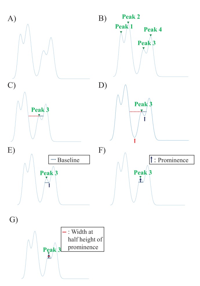Fig. 1

Concept of the width at the half height of the prominence.

(A) The raw data which could be any kind of data, for example, recorded neuronal signal, geological height information, etc. (B) The process of finding local peaks of the signal. (C) Extending horizontal lines from the peak found (peak 3, green arrow head) toward the left (red colored dotted line) and right direction (black colored dotted line). (D) Finding the minimum point of each valley below each horizontal line. (E) Selecting the baseline of peak 3. (F) Defining the height of the prominence (black arrow) of peak 3. (G) Calculating the width at the half height of the prominence.

2. Extend horizontal lines from the peaks found toward the left and right direction until they reach the signal (Fig. 1C).

3. Find the each minimum point of the signal in each horizontal line. (Fig. 1D).

4. The higher valley point defined in the Step 3 specifies the baseline of the topographic prominence (Fig. 1E). The height from this baseline to the peak is the prominence of the peak (Fig. 1F).

For detecting the short-latency responses, we used width at half height of the topographic prominence (Fig. 1G). If the width at half height of a topographic prominence is over 0.4 ms, we consider this peak as a stimulus artifact because the depolarization time of the normal spike is usually within the range of 0.4 ms [27].

Artifact subtraction

Fig. 2 is a flow chart of our signal analysis process for artifact subtraction. First step is stimulation artifact suppression method known as depegging [28]. Our square-shaped stimulus signal induced a huge artifact resembling the stimulus signal shape. This huge artifact does not have any responded spike information from the stimulated RGCs. Therefore, the depegging step sets the stimulus artifact to zero to avoid misinterpreting them as the evoked spikes. After the depegging step, 100 Hz high pass filter is applied for baseline smoothing.

Fig. 2

Flow chart of artifact subtraction.

The depegging step changes saturated artifact value to zero. After the depegging, the remaining signals are filtered with 100 Hz high pass for baseline stabilization. In the process of TP-adopted FB filtering, residual artifacts (over 1.6 ms duration) are separately examined. If the duration at the half height of prominence is under 0.4 ms or if the full duration of the wave is under 1.6 ms, the signal is processed with 500 Hz high pass filtering for spike detection. The signal containing the spike-candidates is then thresholded for spike detection.

Overall, in most previous reports based on frequency filters, these smoothed signals passed through the frequency filters are featured by their own ideas. In our study, before the filtering, the proposed topographic discriminator distinguishes the smoothed signal either to pass through the forward-backward (FB) frequency filter, or just to convert as zero without any filtering.

Specifically, in the smoothed signal, a mountains-like signal over 1.6 ms width is regarded as a residual artifact of the depegged artifact. In here, the mountains-like signal means that a signal starts from a zero level and then ends to zero level having at least one peak. Usually width of the RGC spike is less than 1.6 ms [27]. Therefore, the mountains-like signal over 1.6 ms has much chance embracing one or more RGC spikes. Every peak in the residual artifact is checked whether it is the RGC spike or not using the topographic prominence discriminator, as above described. If the width at the half height of the topographic prominence in the residual artifact is less than 0.4 ms (the usual depolarization time of the RGCs), the peak is regarded as candidates of the evoked RGC spike. This detected peak in the residual artifact is processed by 500 Hz FB high pass filter for thresholding. Under-1.6 ms signal among the mountains-like signal is processed by 500 Hz FB high pass filter for the thresholding as well. On the other hand, wider width of the topographic prominence at half height is considered as noise so that the noise peak is converted to zero. The FB high-pass-filtered signal is investigated by following threshold:

Threshold=4×σ_n

$σ_{n} = m e a n (\frac{|f i l t e r e d s i g n a l|}{0.6745})$

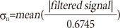
Where σ_n is an estimate of the standard deviation of the background noise. The over-threshold signal is determined as the evoked RGC spike finally.

Receiver operating characteristics

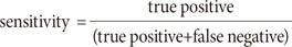
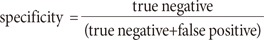
In order to evaluate the proposed topographic prominence discriminator, the discriminated signal was evaluated using the receiver operating characteristics (ROC) analysis. The ROC analysis is one of the most common techniques to visualize the performance of a binary classifier. The ROC organizes decisions of the binary classifiers into four groups: true positive, true negative, false positive, and false negative [29]. The sensitivity and specificity are calculated, as follows:

$sensitivity = \frac{true positive}{(true positive + false negative)}$

$specificity = \frac{true negative}{(true negative + false positive)}$

We evaluated short-latency spike detection performance by comparing the earliest spike of the topographic prominence discriminator with that of only the FB-filtered result without the topographic prominence.

If one algorithm detected a spike within 4 ms after the stimulus had been applied, the result of that algorithm is regarded as the false positive performance. In contrast, if no spike was detected within 4 ms, the result of this algorithm is regarded as the true negative performance. Based on authors' experimental experience, no RGC spikes typically occur within 4 ms after the stimulus so that we utilized 4 ms as a cutoff timing. False positive error rate is calculated, as follows:

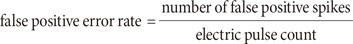
$false positive error rate = \frac{number of false positive spikes}{electric pulse count}$

If one algorithm detected first spike over 4 ms after the stimulus had been applied, the result of that algorithm is regarded as the true positive performance. If the other algorithm detected its own first spike within 2 ms following the earlier spike-detecting algorithm, that algorithm is also considered as having the true positive performance. The 2 ms tolerance window is allowed because the RGC spike is the fast sodium channel-mediated spike typically lasting no more than 2 ms [30]. If an algorithm detects its first spike >2 ms later than the earliest spike, the algorithm is regarded as giving a false negative spike. False negative error rate is calculated, as follows:

$false negative error rate = \frac{number of false negative spikes}{electric pulse count}$

In order to effectively compare and evaluate the TP-adopted FB filter and the only FB filter, we calculated the area under the curve (AUC). The AUC in the ROC defines a quadrangular area composed of (0, 0), (1, 0), (1, 1), and (1 - specificity, sensitivity) in the ROC graph. Larger AUC means better performance.

Retinal preparation

C3H/HeJ strains (rd1 mice) at postnatal week 10 and higher were used for the retinal degeneration model (number of mouse=3). At this postnatal age, the retinas are no longer responsive to light, but extensive remodeling of the inner retina has not yet occurred. Instead, functional stability of RGCs is well preserved up to PNW 30 [31]. All mice were purchased from the Jackson Laboratories (Bar Harbor, ME, USA) and were maintained on a 12-hour light/dark cycle. All experimental methods and animal care procedures were approved by the institutional animal care committee of Chungbuk National University (approval number: CBNURA-042-0902-1). Details of the method of retinal patch preparation and stimulation used in our laboratory may be found in [9]. After eliciting short- and long-latency RGC spikes by electrical stimulation, the long-latency spikes (which are network mediated through synaptic transmission), were blocked by application of a Ca²⁺-channel blocker, cadmium chloride (CdCl₂; 20 µM). We only showed CdCl₂-treated, long-latency spike blocked data in this article.

Electrode and data recording system

The data acquisition system (MEA60 system; Multi Channel Systems GmbH, Reutlingen, Germany) included planar MEA, stimulator (STG1004), amplifier (MEA1060), temperature control units, data acquisition hardware (Mc_Card) and software (Mc_Rack). The MEA contained 64 circular-shaped electrodes in an 8×8 grid layout with electrode diameters of 30 µm and interelectrode distances of 200 µm. The electrodes are coated with porous titanium nitride (TiN) to minimize electrical impedance. The four electrodes at the vertices were inactive. Multi-electrode recordings of the retinal activity were obtained from 60 electrode channels with a bandwidth ranging from 1 to 3,000 Hz at a gain of 1,200. The data sampling rate was 25 kHz/channel. No light was applied for these experiments and spontaneous retinal activity was recorded.

Electrical stimulation

Using a stimulus generator (STG 1004, Multichannel systems GmbH, Germany), current pulse trains were delivered to the retinal preparation via one of the 60 channels (mostly channel 44 in the middle of the MEA). The remaining channels of the MEA were classified into four groups by distances between the stimulus and recording electrodes on MEA (200~400, 400~600, 600~800, 800~1000 µm) (Fig. 3A). The stimuli consisted of symmetric cathodic phase-1^st biphasic pulses. We fixed pulse duration at 500 µs and applied pulse amplitude at 5, 10, 20, 30, 40, 50, 60 µA. Biphasic current pulses were applied once per second (1 Hz, ×50 times) (Fig. 3B).

Fig. 3

MEA recording and electrical stimulation.

(A) One electrode was used for stimulation (asterisk in the center), while all the others for recording. The recorded signals were classified into four groups by distances between the stimulus and recording electrodes on MEA (200~400, 400~600, 600~800, 800~1000 µm). (B) The stimuli consists of cathodic phase-1st biphasic current pulses (Duration (D): 500 µs, Amplitude intensity (A): 5, 10, 20, 30, 40, 50, 60 µA, Inter-stimulus interval (I): 1000 ms, Repetition (R): 50 times).

Go to :

RESULTS

Comparison of false positive error at 200~400 µm inter-electrode distance

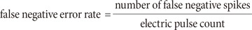
We compared false positive error and false negative error in FB filter and TP-adopted FB filter. With FB filter, there remained huge stimulus artifact and artifact-induced false positive spike, on the other hand, TP-adopted FB filter subtracted an artifact good enough to isolate true spike in current intensity of 10 µA (Fig. 4A). By increasing current intensity to 30 µA, both FB filter and TP-adopted FB filter showed false positive spikes (Fig. 4B). However, the number of false positive spikes is different; 2 vs. 1 in FB filter vs. TP-adopted FB filter. Statistical analysis showed that TP-adopted filter significantly decreased the number of false positive spikes throughout all stimulus intensity except 50 µA (Fig. 4C).

Fig. 4

Comparison of false positive error at 200~400 µm inter-electrode distance.

(A, B) The performance of two algorithms at stimulus intensity of 10 µA and 30 µA were shown respectively. The thin and thick lines represent raw signal, and filtered output (artifact-subtracted) signal respectively. The dotted line represents threshold value for sorting RGC spikes from noise. The arrows indicate false positive spikes (Inset: true positive spike). (C) False positive error rates (false positive spikes/pulse) of two algorithms were statistically analyzed at all stimulus intensities.

Comparison of false negative error at 200~400 µm inter-electrode distance

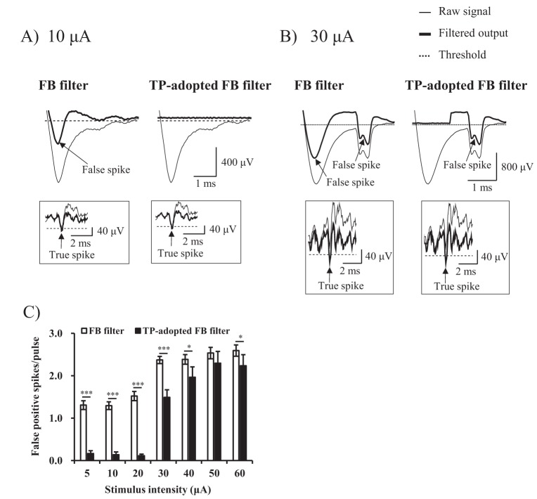
At current intensity of 10 µA, FB filter detected a true spike, while TP-adopted FB filter missed the true spike, in other words, it had false negative error (Fig. 5A). At current intensity of 30 µA, both FB filter and TP-adopted FB filter missed the true spike. However, the number of false negative spike was less with FB filter than TP-adopted filter (0 vs. 1) (Fig. 5B). Statistical analysis showed that TP-adopted FB filter missed true spikes more significantly than FB filter throughout all current intensities (Fig. 5C) (5~10 µA: p<0.01, 20~60 µA: p<0.001). In spite of statistical differences between two artifact subtraction methods, the numerical value of false negative spikes was still considerably under one with TP-adopted FB filter (e.g. average false negative spikes per pulse at 30 µA was 0.17). It means that the probability with which TP-adopted FB filter mistakes a true spike as an artifact is 0.17, on the contrary, probability of finding a true spike is 1 minus 0.17 (0.83) at minimum. The false negative error of TP-adopted FB filter was very small compared with false positive error of FB filter which was more than one throughout all current intensities (Fig. 4C).

Fig. 5

Comparison of false negative error at 200~400 µm inter-electrode distance.

(A, B) The performance of two algorithms at stimulus intensity of 10 µA and 30 µA were shown respectively. The thin and thick lines represent raw signal, and filtered output (artifact-subtracted) signal respectively. The dotted line represents threshold value for sorting RGC spikes from noise (Symbols: arrow=true positive spike). (C) False negative error rates (false negative spikes/pulse) of two algorithms were statistically analyzed at all stimulus intensities (Inset: To view false negative error rates of FB filter, the scale was zoomed in).

Comparison of false positive and false negative error according to incremental distances of electrodes

When inter-electrode distance between stimulus electrode and recording electrodes is apart more than 400 µm, false positive error of FB filter remained more than one spike per pulse and it was substantially larger than that of TP-adopted FB filter throughout all current intensities (p<0.001) (Figs. 6C-6E). On the other hand, false negative error of TP-adopted FB filter declined from 0.17 to 0.08, 0.06, and 0.05 at inter-electrode distance of 200~400, 400~600, 600~800, and 800~1000 µm, respectively (Figs. 7C-E).

Fig. 6

Comparison of false positive error according to incremental distances of electrodes.

(A, B) The performance of two algorithms at stimulus intensity of 10 µA and 30 µA were shown respectively at 600~800 µm inter-electrode distance. The thin and thick lines represent raw signal, and filtered output (artifact-subtracted) signal respectively. The dotted line represents threshold value for sorting RGC spikes from noise. The arrows indicate false positive spikes (Inset: true positive spike). (C~E) False positive error rates (false positive spikes/pulse) of two algorithms at all stimulus intensities were statistically analyzed in terms of inter-electrode distance.

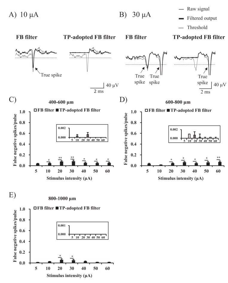Fig. 7

Comparison of false negative error according to incremental distances of electrodes.

(A, B) The performance of two algorithms at stimulus intensity of 10 µA and 30 µA were shown respectively at 600~800 µm inter-electrode distance. The thin and thick lines represent raw signal, and filtered output (artifact-subtracted) signal respectively. The dotted line represents threshold value for sorting RGC spikes from noise (Symbols: arrow=true positive spike). (C~E) False negative error rates (false negative spikes/pulse) of two algorithms at all stimulus intensities were statistically analyzed in terms of inter-electrode distance (Inset: To view false negative error rates of FB filter, the scales were zoomed in).

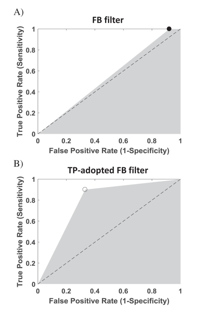
Comparison of AUC graphs

We calculated AUC value to compare each method's artifact subtraction performance (Fig. 8). The AUC value with FB filter and TP-adopted FB filter was 0.54 and 0.79, respectively. Because ROC analysis comprehensively represents sensitivity and specificity and larger AUC means better performance, TP-adopted FB filter shows better performance than FB-filter alone.

Fig. 8

Area under the curve (AUC ) graph.

(A, B) The AUC graphs of two algorithms were displayed. The areas of grey quadrangle represent AUC value.

Go to :

DISCUSSION

Advantages of the adoption of topographic prominence discriminator

The concept of topographic prominence originates in geology and geography for calculating heights of local peaks [26]. In this study, we proposed the prominence discriminator to separate the spike from the stimulus artifact by computing their widths. The prominence discriminator has several advantages: First, it can separate the spikes from the stimulus artifacts without further manipulation including pharmacological experiment [13 18 19], or subtraction between responses of over-threshold stimulation and under-threshold stimulation [13 32]. Second, the prominence discriminator increases performance to remove stimulus artifacts. The frequency-based filters have not shown good performance for depressing the stimulus artifacts [28], because these stimulus artifacts have diverse amplitude and frequency. When the prominence discriminator is added to FB-filter, it helps the frequency-based FB filter remove the stimulus artifacts better (Fig. 8).

When a priori knowledge on the features of artifacts is not available, or when the shape and size of them vary for each stimulus, it has been known to be a tricky problem to distinguish artifacts from spikes. Because stimulus artifact tends to coincide with the short-latency spikes which usually occur within 4~10 ms of the stimulus start. Therefore, it is difficult to isolate the shortlatency spikes from stimulus artifact.

Several artifacts subtraction algorithms reported in the literature including TTX subtraction based on pharmacological manipulation [13 18 19], template subtraction [20], sample-andinterpolate technique [21], and independent component analysis assumed the same shape of artifacts for repetitive stimulation [33]. We present a new method which is robust to the change of duration and height of the artifacts, the prominence discriminator. It can be additionally used with a traditional high-pass filter like forward and backward (FB) filter as shown in Fig. 2. In order to verify the feasibility (usefulness) of the proposed method, we conducted several experiments on subtracting artifacts using FB filter only and FB filter with the prominence discriminator and compared the performance statistically.

Comparison of the topographic discriminator-adopted filter with the only frequency-based filter

We wanted to see whether the prominence discriminator method could increase the performance of the FB filter regardless of the strength of stimulus and the configuration of MEA. When we increased the current on the stimulus electrode from 10 to 50 µA by 10 µA, the false positive errors also increased for each filter. However, the FB filter with the prominence discriminator shows the better performance under all the conditions. The experiments for performance comparison showed that the prominence discriminator could improve the performance of the traditional frequency-based filter in subtracting artifacts for short-latency spikes.

Inter-electrode distance between stimulus and recording electrodes affects false negative error

Shapes of the stimulus artifacts differ according to distance between the stimulus electrode and the recording electrodes. When we changed the distance between the electrodes from 200 to 1000 µm by 200 µm, the false negative errors decreased. Because we used single channel of MEA as stimulus electrode, the further distance between stimulus and recording electrodes is, the smaller the stimulus current becomes. Therefore, the stimulus artifact becomes smaller on further recording electrodes and smaller artifact can hardly obfuscate the spike. On the other hand, RGC spike amplitude only depends on the distance between the location of RGC and the recording electrode not the distance between stimulus and recording electrodes. Therefore, eventually the chance of false negative error decreases with increment of interelectrode distance (Figs. 7C-E).

Future works

Even though the prominence discriminator can improve the performance of traditional artifact subtraction algorithms in view of the false positive error, this is not saying that the performance of neural encoding of retinal ganglion cell can be improved as much as the identical rate with the improvement of the false positive error. If this prominence discriminator algorithm can be applied in real time basis, this could improve the spike detection accuracy greatly. We would like to pursue real time basis-adoption of TP discriminator in our future research.

Go to :

ACKNOWLEDGEMENTS

This work was supported by Goo's grants (NRF-2015R1D1A1A01056903, NRF-2017M3A9E2056460, research grant of the Chungbuk National University in 2014) and Koo's grants of the Ministry of Science, ICT & Future, Planning (NRF-2017R1DA1A1B03034982 & NRF-2017M3A9E2062707).

Go to :

Notes

Author contributions: J.R.A., M.H.C., K.I.K., and Y.S.G. conceived and designed the experiments; J.R.A. and M.H.C. performed experiments; J.R.A., M.H.C., K.S.K, S.S.S, and D.Cho analyzed the data; J.R.A, K.I.K, Y.S.G. wrote the manuscript.

CONFLICTS OF INTEREST: The authors declare no conflicts of interest.

Go to :

References

1. Shintani K, Shechtman DL, Gurwood AS. Review and update: current treatment trends for patients with retinitis pigmentosa. Optometry. 2009; 80:384–401. PMID: 19545852.

2. Mehta S. Age-related macular degeneration. Prim Care. 2015; 42:377–391. PMID: 26319344.

3. Kim SY, Sadda S, Pearlman J, Humayun MS, de Juan E Jr, Melia BM, Green WR. Morphometric analysis of the macula in eyes with disciform age-related macular degeneration. Retina. 2002; 22:471–477. PMID: 12172115.

4. Mazzoni F, Novelli E, Strettoi E. Retinal ganglion cells survive and maintain normal dendritic morphology in a mouse model of inherited photoreceptor degeneration. J Neurosci. 2008; 28:14282–14292. PMID: 19109509.

5. Santos A, Humayun MS, de Juan E Jr, Greenburg RJ, Marsh MJ, Klock IB, Milam AH. Preservation of the inner retina in retinitis pigmentosa A morphometric analysis. Arch Ophthalmol. 1997; 115:511–515. PMID: 9109761.

6. Stone JL, Barlow WE, Humayun MS, de Juan E Jr, Milam AH. Morphometric analysis of macular photoreceptors and ganglion cells in retinas with retinitis pigmentosa. Arch Ophthalmol. 1992; 110:1634–1639. PMID: 1444925.

7. Stingl K, Bartz-Schmidt KU, Besch D, Chee CK, Cottriall CL, Gekeler F, Groppe M, Jackson TL, MacLaren RE, Koitschev A, Kusnyerik A, Neffendorf J, Nemeth J, Naeem MA, Peters T, Ramsden JD, Sachs H, Simpson A, Singh MS, Wilhelm B, Wong D, Zrenner E. Subretinal visual implant alpha IMS−clinical trial interim report. Vision Res. 2015; 111:149–160. PMID: 25812924.

8. Luo YH, da Cruz L. The argus® II retinal prosthesis system. Prog Retin Eye Res. 2016; 50:89–107. PMID: 26404104.

9. Ahn KN, Ahn JY, Kim JH, Cho K, Koo KI, Senok SS, Goo YS. Effect of stimulus waveform of biphasic current pulse on retinal ganglion cell responses in retinal degeneration (rd1) mice. Korean J Physiol Pharmacol. 2015; 19:167–175. PMID: 25729279.

10. Boinagrov D, Pangratz-Fuehrer S, Goetz G, Palanker D. Selectivity of direct and network-mediated stimulation of the retinal ganglion cells with epi-, sub- and intraretinal electrodes. J Neural Eng. 2014; 11:026008. PMID: 24608166.

11. Jensen RJ, Ziv OR, Rizzo JF 3rd. Thresholds for activation of rabbit retinal ganglion cells with relatively large, extracellular microelectrodes. Invest Ophthalmol Vis Sci. 2005; 46:1486–1496. PMID: 15790920.

12. Lee SW, Eddington DK, Fried SI. Responses to pulsatile subretinal electric stimulation: effects of amplitude and duration. J Neurophysiol. 2013; 109:1954–1968. PMID: 23343891.

13. Sekirnjak C, Hottowy P, Sher A, Dabrowski W, Litke AM, Chichilnisky EJ. Electrical stimulation of mammalian retinal ganglion cells with multielectrode arrays. J Neurophysiol. 2006; 95:3311–3327. PMID: 16436479.

14. Stett A, Barth W, Weiss S, Haemmerle H, Zrenner E. Electrical multisite stimulation of the isolated chicken retina. Vision Res. 2000; 40:1785–1795. PMID: 10814763.

15. Im M, Fried SI. Indirect activation elicits strong correlations between light and electrical responses in ON but not OFF retinal ganglion cells. J Physiol. 2015; 593:3577–3596. PMID: 26033477.

16. Grumet AE. Electric stimulation parameters for an epi-retinal prosthesis. (dissertation). Department of Electrical Engineering and Computer Science, Cambridge, MA: Massachusetts Institute of Technology;1999.

17. Nagel JH. Biopotential amplifiers. In : Bronzino JD, editor. The biomedical engineering handbook. Boca Raton: CRC Press;1995. p. 1185–1195.

18. Fried SI, Hsueh HA, Werblin FS. A method for generating precise temporal patterns of retinal spiking using prosthetic stimulation. J Neurophysiol. 2006; 95:970–978. PMID: 16236780.

19. Ryu SB, Ye JH, Lee JS, Goo YS, Kim CH, Kim KH. Electrically-evoked neural activities of rd1 mice retinal ganglion cells by repetitive pulse stimulation. Korean J Physiol Pharmacol. 2009; 13:443–448. PMID: 20054490.

20. Miller CA, Abbas PJ, Robinson BK, Rubinstein JT, Matsuoka AJ. Electrically evoked single-fiber action potentials from cat: responses to monopolar, monophasic stimulation. Hear Res. 1999; 130:197–218. PMID: 10320109.

21. Heffer LF, Fallon JB. A novel stimulus artifact removal technique for high-rate electrical stimulation. J Neurosci Methods. 2008; 170:277–284. PMID: 18339428.

22. Erickson JC, Velasco-Castedo R, Obioha C, Cheng LK, Angeli TR, O'Grady G. Automated algorithm for GI spike burst detection and demonstration of efficacy in ischemic small intestine. Ann Biomed Eng. 2013; 41:2215–2228. PMID: 23612912.

23. Killian NJ, Vernekar VN, Potter SM, Vukasinovic J. A device for long-term perfusion, imaging, and electrical interfacing of brain tissue in vitro. Front Neurosci. 2016; 10:135. PMID: 27065793.

24. Pan L, Alagapan S, Franca E, Leondopulos SS, DeMarse TB, Brewer GJ, Wheeler BC. An in vitro method to manipulate the direction and functional strength between neural populations. Front Neural Circuits. 2015; 9:32. PMID: 26236198.

25. Choi MH, Ahn J, Park DJ, Lee SM, Kim K, Cho DD, Senok SS, Koo KI, Goo YS. Topographic prominence discriminator for the detection of short-latency spikes of retinal ganglion cells. J Neural Eng. 2017; 14:016017. PMID: 28045002.

26. Llobera M. Building past landscape perception with GIS: understanding topographic prominence. J Archaeol Sci. 2001; 28:1005–1014.

27. Bullock TH, Horridge AG. Structure and function in the nervous systems of invertebrates. San Francisco, London: W. H. Freeman & Co.;1965.

28. Wagenaar DA, Potter SM. Real-time multi-channel stimulus artifact suppression by local curve fitting. J Neurosci Methods. 2002; 120:113–120. PMID: 12385761.

29. Fawcett T. An introduction to ROC analysis. Pattern Recognit Lett. 2006; 27:861–874.

30. Kuffler SW. Discharge patterns and functional organization of mammalian retina. J Neurophysiol. 1953; 16:37–68. PMID: 13035466.

31. Margolis DJ, Newkirk G, Euler T, Detwiler PB. Functional stability of retinal ganglion cells after degeneration-induced changes in synaptic input. J Neurosci. 2008; 28:6526–6536. PMID: 18562624.

32. Li L, Hayashida Y, Yagi T. Temporal properties of retinal ganglion cell responses to local transretinal current stimuli in the frog retina. Vision Res. 2005; 45:263–273. PMID: 15581924.

33. Lu Y, Cao P, Sun J, Wang J, Li L, Ren Q, Chen Y, Chai X. Using independent component analysis to remove artifacts in visual cortex responses elicited by electrical stimulation of the optic nerve. J Neural Eng. 2012; 9:026002. PMID: 22306622.

Go to :

TOOLS

Similar articles