

 PDF
PDF ePub
ePub Citation
 Print
Print


INTRODUCTION
Parkinson's disease (PD) is a neurodegenerative disorder that causes considerable movement disability. It is well known that motor symptoms of PD are caused by the death of dopamine-generating cells in the pars compacta region of the substantia nigra. To reverse parkinsonian symptoms, pharmacological therapy using levodopa (L-dopa) has been used, as L-dopa is converted into dopamine in the brain [1]. However, drugs eventually become ineffective due to the gradual loss of dopaminergic neurons as the disease progresses. Surgical treatments, such as lesioning specific parts of the brain and deep brain stimulation (DBS), have been used as alternatives.
The stimulation of the STN by electrical pulses has now been accepted as a practical treatment for PD-related movement disorders, including tremor and dystonia [2-8]. Several reports on neural activities evoked by DBS can be found in the literature [9-13], yet the mechanism of DBS is not clearly understood. Contradictory results exist on the effect of DBS; it is unclear whether the STN DBS produces an inhibitory or excitatory effect. For example, Benabid et al. reported that high frequency DBS can mimic the effects of lesioning [14,15]. Benazzouz et al. showed that STN stimulation can cause inhibition of the STN excitatory output [9,10]. However, Vitek et al. reported that lesions and DBS could produce the opposite effects [16]. In addition, Windels et al. demonstrated that high frequency stimulation of STN could increase firing of STN neurons [17]. These contradictions may be due to differences in the details of stimulation parameters or differences in experimental protocols. However, it is more likely that STN DBS could induce more complex responses in the basal ganglia (BG). Shi et al. reported that BG neurons of GP and substantia nigra pars reticulate (SNr) showed both inhibitory and excitatory responses while behaviorally effective DBS was delivered to the STN. These results indicate that the therapeutic effect of DBS might not be caused by a simple inhibition or excitation of the BG [18]. Therefore, investigations of neuronal activity in relevant areas in the BG as well as the stimulated area are essential to clarify DBS mechanism.
Electrical stimulation produces large artifact waveforms whenever neural recordings are performed simultaneously with electrical stimulation. The artifacts significantly occlude or completely block neural spike waveforms. To resolve this issue, several artifact removal techniques have been devised [19-23]. Most artifact removal techniques employ a template subtraction method that attempts to reconstruct spike waveforms by subtracting a mean artifact waveform from each recorded artifact waveform. These techniques could generate residual artifacts due to the variability in the stimulation onset time or the variation in artifact waveforms. To alleviate this problem, we developed a custom artifact removal technique using a curve-fitting method to minimize possible residual artifacts by generating a template from a single artifact waveform. Simulations that test spike detection and classification from artifact-removed signals validated the developed artifact removal technique.
In this study, using the custom artifact removal technique, we aimed to observe changes of neuronal activities in the GP of normal and Parkinson's disease model rats while electrical stimulation was applied to the STN. Because it is known that the therapeutic effects of DBS are strongly dependent on the stimulation frequency, we investigated how the frequency of STN stimulation affects neuronal activities in the GP.
Go to : 
METHODS
Animal preparation
A total of 5 adult male Sprague-Dawley rats (200~250 g) were used. Rats were divided into two groups as follows: (i) a normal control group containing 2 rats without lesions and (ii) a PD model group containing 3 rats with a medial forebrain bundle (MFB) lesion induced by 6-hydroxydopamine (6-OHDA). Rats with MFB lesion has been proposed as a good model of the akinesia associated with PD because it induced deficits in forepaw adjusting steps in rats [24]. To explain briefly, rats were anesthetized with a mixture of ketamine (75 mg/kg), acepromazine (0.75 mg/kg) and xylazine (4 mg/kg), and mounted on a stereotaxic apparatus. 6-OHDA hydrobromide (8 µg free base in 0.2% ascorbic acid, Sigma, St. Louis, MO) was injected unilaterally into the MFB according to the following stereotaxic coordinates: AP -4.4 mm, ML 1.2 mm relative to bregma, and DV -7.5 mm from the dura mater. In 6-OHDA injection, we made the injection needles using stainless steel pipe (in 200 µm diameter). The needles were sanitizes with E.O. gas and connected with Hamilton microsyringe (80330, Hamilton company, Reno, NV, U.S.A). The solution was injected at a rate of 0.5 µl/min using a cannula and the injection was pushed by hand. A polyethylene tube was used to connect the cannula and microsyringe. To prevent noradrenergic neurons from being destroyed, desipramine (12.5 mg/kg, intraperitoneally) was administered 30 min prior to the 6-OHDA infusion. Electrophysiological recordings were performed 5 weeks after the 6-OHDA lesion.
Extracellular recording and electrical stimulation
Extracellular recordings of single unit activities from rats were performed under anesthesia with a mixture of Zoletil 50 (40 mg/kg) and xylazine (9 mg/kg). A microelectrode (A-M systems, Tungsten, diameter: 0.005 in, AC impedance 5 MΩ, product no. 573400) was used for the recording. The microelectrode was stereotaxically guided through a burr hole drilled in the skull at the target coordinates (GP, AP, -0.92 mm; ML, 3 mm; DV, 6.0~6.6 mm). A charge-balanced biphasic current pulse train was generated by a stimulator (A-M systems, isolated pulse stimulator, model 2100) and applied to the subthalamic nucleus (STN, AP, -3.7 mm; ML, 2.5 mm; DV, 7.4~7.8 mm) through a stimulation electrode (A-M systems, Tungsten, diameter: 0.010 in, tip exposure: 1 mm, product no.563410) with amplitudes of 100 and 200 µA, and a pulse duration of 60 µs. Stimulation frequency was varied from 10 to 130 Hz (10, 50, 90 and 130 Hz). Electrical signals were amplified using an amplifier (A-M systems, microelectrode AC amplifier, model 1800). The signals were stored on a PC equipped with Spike 2 software (version 2.18, Cambridge Electronic De sign, UK) and analyzed by using Matlab (Mathwork, USA).
Artifact removal and data analysis
Fig. 1A shows a typical waveform recorded from the GP during electrical stimulation applied to the STN. Although it is possible to observe spikes during the fluctuation of the artifact waveform by adjusting the time and amplitude scale, it is not easy to detect spikes by an amplitude threshold (Fig. 1B). To remove the fluctuation and detect spikes, a template for the artifact subtraction was constructed by a curve-fitting method. As shown in Fig. 1C, the artifact waveform of the trace in Fig. 1B was divided into several segments and each segment is curve-fitted with a 2nd to 4th order polynomial. The length of each segment is adjusted according to the shape of the segment; usually a 50~100 sample length (2~4 ms) was appropriate in the present study. The order of the polynomial was decided not to curve-fit the spike waveform in the artifact. After all the segments were curve-fitted, the segments were gathered to construct a template (Fig. 1C). For our experimental data, a period of 2 ms from the stimulation onset was flattened because the artifact waveform is saturated, and spikes cannot be detected in this period. For the final step, the constructed template was subtracted from the original artifact waveform. As a result, the artifact waveform and the fluctuation were effectively removed and spikes were clearly revealed (Fig. 1D and Fig. 2). This procedure was repeated for all the artifact waveform and finally, the artifact-free neural signal could be obtained (Fig. 1E). After the artifacts were removed, spikes were detected and sorted by the principal component analysis (PCA) as shown in Fig. 3C. To quantitatively assess changes in neuronal activities with electrical stimulation, firing rate before and during the electrical stimulation was calculated and compared.
 | Fig. 1Protocol for artifact removal with a curve-fitting method. (A) Single unit activities are covered by large stimulus artifact waveforms. (B) An example of one artifact waveform at a stimulation frequency of 10 Hz. Several spikes were mixed on the fluctuation generated by an artifact waveform (indicated by arrows). (C) The artifact waveform is divided into several segments and each segment is curve-fitted with 2nd to 4th order polynomial. Every curve-fitted waveform is gathered together to construct a template for artifact subtraction. (D) Spike waveforms were clearly revealed after artifact subtraction (the template is subtracted from the original waveforms). (E) Every artifact waveform is subtracted by templates, which are curve-fitted from their own waveform. After this procedure is repeated, an artifact-removed signal is obtained.
|
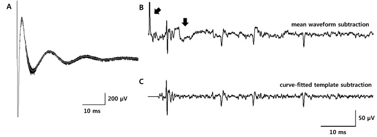 | Fig. 2Comparison of two artifact removal methods. (A) 100 overlapped artifact waveforms (thick gray trace: mean waveform) recorded with a stimulation frequency of 10 Hz. (B) Artifact-removed waveform after the mean waveform subtraction. Residual artifacts and fluctuation remained (indicated by arrows). (C) Artifact-removed waveform after the template subtraction with the curve-fitting method. Residual artifacts that are shown in Fig. 2 (B) were not generated using the curve-fitting method.
|
 | Fig. 3Simulations for the validation of the effectiveness of the artifact removal technique with the curve-fitting method. (A, B) Two different shapes of spikes were randomly synthesized to the noise (first 20 seconds) and to the noise and artifact waveforms (second 20 seconds). In this figure, stimulation frequency of the artifacts was 90 Hz (top: before artifact removal, bottom: after artifact removal). (C) Spikes are detected after artifact removal and classified by principal component analysis (PCA). Spikes detected before and after artifact subtractions have similar spike waveforms and can be reliably classified into two groups (In the box: spikes waveforms sorted by PCA analysis. Black waveforms: spikes detected from the first 20 seconds. Grey waveforms: spikes detected from the second 20 seconds after artifacts were removed).
|
Go to :
RESULTS
Simulation of artifact removal
To validate the effectiveness of our custom artifact removal, a simulation was performed to detect and classify spikes under conditions when spikes were mixed with artifact waveforms. For the simulation, stimulation artifact waveforms (of various stimulation frequencies: 10, 50, 90 and 130 Hz) and two different shapes of spike waveforms (two units) were extracted from an experimental dataset. The simulation consisted of control and test sessions. The control session was 20 seconds long, and two different spike waveforms were randomly synthesized on the noise (the total number of spikes is 800 which means that 400 spikes per unit were used in the simulation). The test session was also 20 seconds long, and two different spike waveforms were randomly synthesized on the noise signal and on the stimulation artifact waveforms, avoiding each stimulation onset (Fig. 3A, top). After the signal for the simulation was generated, artifact waveforms were removed by the artifact removal technique (Fig. 3A and 3B). Spikes were detected by threshold and sorted by their waveforms using the principal component analysis (Fig. 3C). Although the amplitudes of some spikes were diminished in size, they were reliably classified into two groups. The simulation was repeated 10 times for each stimulation frequency and the accuracy was calculated by checking whether the timestamps of detected spike trains were correct. As shown in Table 1, the average accuracy of detected spikes was approximately 80~90%, which means that over 80% of spikes were successfully detected from artifact-contaminated waveforms.

Responses of GP neurons during STN stimulation
Fig. 4 shows response characteristics of a GP neuron in a PD model rat to electrical stimulation of the STN. As shown in Fig. 4A, inhibitory periods followed stimulation pulses and stronger stimulation induced longer inhibition (top: 100 µA, bottom: 200 µA). When an electrical pulse was applied repeatedly 50 times with a 5 s interval, inhibition was consistently observed in the raster plot (Fig. 4C). From the poststimulus time histogram (PSTH) in Fig. 4B, it was found that the duration of the inhibitory period was approximately 100 and 200 ms when the pulse amplitude was 100 µA and 200 µA, respectively.
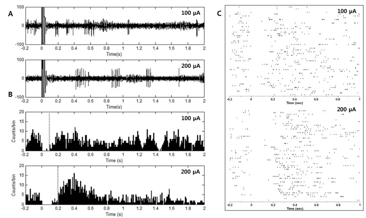 | Fig. 4Inhibition of neuronal activity of GP neurons by STN stimulation. (A) Inhibition of neuronal activity followed electrical stimulation. Stimulation of a larger amplitude induced longer inhibition (top: 100 µA, bottom: 200 µA). (B, C) A post-stimulus time histogram (PSTH, time bin: 10 ms) and raster plot were constructed from 50 repetitive stimulations. The duration of the inhibition was approximately 100 ms and 200 ms for pulse amplitude 100 µA and 200 µA, respectively.
|
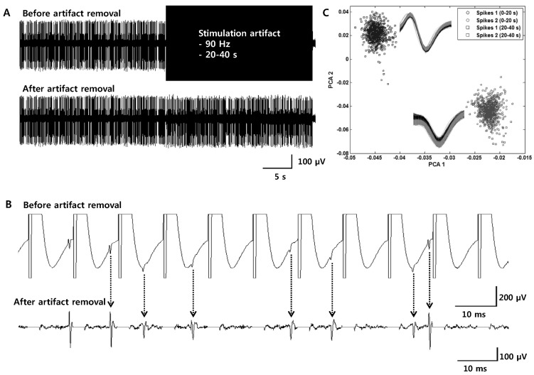
Fig. 5A demonstrates neural activities of GP neurons in a PD model rat, recorded with stimulation artifacts. Because it is impossible to observe spikes during STN stimulation due to these stimulation artifacts, the artifacts were eliminated with the artifact removal technique. After artifact removal, spikes were detected and classified into two units (Fig. 5B and 5C). As seen in Fig. 5B, spikes with large amplitudes were modulated by high-frequency STN stimulation and significantly suppressed when stimulation frequency was over 50 Hz (This result is demonstrated in Table 2, PD Cell 1).
 | Fig. 5Waveforms recorded from GP neurons of Parkinson's disease model rats. (A) Electrical stimulations were applied to the STN with various stimulation frequencies (from the top: 10, 50, 90 and 130 Hz). (B) Artifact-removed waveforms. Artifact-removed periods are indicated with boxes of dotted lines. (C) Spike waveforms detected from each waveform. Two units were detected and sorted. Spikes with amplitude larger than another unit showed inhibition of firing rate when high frequency stimulation was applied to the STN.
|

To quantitatively assess changes in the firing rate due to STN stimulation, we calculated and compared relative changes in the firing rate between two periods- the 10 s preceding stimulation and during the 10 s stimulation. As shown in Fig. 6, the relative change in the firing rate of GP cells decreased according to the stimulation frequency. In order to check whether its change was significant, statistical test was performed for every cell in PD model rats (Table 2). It was found that the firing rate was significantly decreased when the STN was electrically stimulated with frequency higher than 50 Hz.
 | Fig. 6Changes in the firing rate according to the stimulation frequency. Changes of the mean firing rate during electrical stimulation were compared to the mean firing rate 10 s before the stimulation to obtain quantitative values (relative change, %). Both in (A) normal and (B) PD model rat, significant inhibition of neuronal firing was observed at stimulation frequencies higher than 50 Hz.
|
Go to :
DISCUSSION
In the present study, we observed neuronal activities in the GP of normal and PD model rats responding to STN stimulation. According to the traditional model of the BG-thalamocortical network [25], the pathophysiological mechanisms underlying movement disorders of PD are associated with abnormal outflows within the BG. It is regarded that neuronal responses within the BG directly reflect the effect of STN stimulation. Therefore, characterizing BG neuron responses can help us understand the working mechanism of DBS. We specifically focused on observing GP neuronal activities during STN stimulation using a custom artifact removal technique and demonstrated how responses changed with the frequency of STN stimulation.
Previous studies mainly investigated neuronal responses that occurred after the termination of electrical stimulation with the assumption that neuronal activities following the stimulation may reflect activities that occurred during stimulation [9,10]. However, Montgomery et al. [26] demonstrated that increased neuronal activities during electrical stimulation were reduced after the cessation of the stimulation, implying that neuronal activities following electrical stimulation may show an effect opposite to that which occurs during the stimulation. Accordingly, the observation of neuronal activities during electrical stimulation is regarded as an important tool for the study of the mechanism of DBS.
Single pulse stimulation of the STN induced inhibitory responses in the GP (Fig. 4). However, the inhibitory effect was very brief and recovered quickly and it is not expected that a single pulse can generate clinical effects. We observed neural activities in the GP responding to a pulsetrain stimulation of the STN under various stimulation frequencies. GP activity was not significantly suppressed in PD model rats when the stimulation frequency was as low as 10 Hz. However, GP activity was remarkably inhibited when the stimulation frequency increased to be greater than 50 Hz (Fig. 6, Table 2). This result supports the indirect inhibition of pathological activity hypothesis [27], which suggests that high-frequency stimulation is effective because there is less opportunity for abnormal neuronal activity to return to the baseline pathological activity due to the short inter-stimulus pulse intervals. A stimulation frequency of 50 Hz may be inconsistent with generally accepted stimulation parameters such as 130 Hz. However, as shown in the results of the single pulse stimulation, neuronal activities are affected not only by stimulation frequency but also by stimulation intensity. Thus, for a direct comparison of the results on stimulation frequency, other conditions such as stimulation intensity, pulse width, stimulation period and subjects group should be matched. Nevertheless, our results are in good agreement with the results of Limousin et al. [5], which demonstrated that a beneficial effect of STN stimulation on parkinsonian motor symptoms was dependent on stimulation frequency and the maximum effect occurs over 50 Hz. Therefore, we hypothesize that STN stimulation could be effective for the alleviation of parkinsonian symptoms when the stimulation parameter is strong enough to inhibit neuronal activities.
We used an artifact removal technique devised from a curve-fitting method as an essential tool in this study. Stimulation artifact is a major problem in the study of neuronal activities responding to the high-frequency electrical stimulation as artifact waveforms not only occupy most of the recording time but also occlude neural signals. Several studies employed a template subtraction method that subtracts a mean artifact waveform (template waveform) from each artifact waveform and showed that is effective for revealing spikes occluded by artifact waveforms. However, when we tested the template subtraction method using a mean artifact waveform, there were unintended residual artifacts and fluctuations left after the subtraction (Fig. 2B). Although residual artifacts due to the variation of the stimulation onset can be removed by flattening the short segment before and after the stimulation onset, residual fluctuations cannot be easily flattened because the length of the fluctuation may be long enough to contain spikes. This may be the reason why Hashimoto et al. [20] emphasized that it is critically important to construct an accurate template for this method. Another possible problem is having evoked spikes with a fixed latency. If spikes are evoked with a fixed latency responding to the stimulation, a template constructed by averaging artifact waveforms may contain the spike shape in the template and can eliminate each evoked spike by the template subtraction. Our artifact removal technique was devised to avoid the problems of the mean waveform subtraction. Because the template is generated from a single artifact waveform by curve-fitting each waveform, it can minimize the variance between the template and each artifact waveform and, therefore, prevent the residual artifacts. This was most effective when the stimulation frequency was low so that the length of an artifact waveform was several tens of milliseconds. In addition, it could reduce the concern for the elimination of spikes with a fixed latency, as the template is generated to fit each artifact waveform. Moreover, this method can be applied not only to sequential pulse-trains but also to single pulses because it is not necessary to collect many artifact waveforms to construct an average waveform template.
Here, we observed that neuronal activities of the GP are inhibited by high frequency STN stimulation. However, it is still necessary to investigate neuronal responses of other BG neurons as well as the cortex to understand the mechanism. Therefore, in future studies, simultaneous multichannel recording from the BG and the cortex should be performed during electrical stimulation. Observation of single unit activity as well as local field potentials from various sites within the BG will also provide valuable information about the mechanism of DBS.
Go to :
 XML Download