

 PDF
PDF ePub
ePub Citation
 Print
Print


INTRODUCTION
Depression is a significant public health concern and contributes substantially to the global burden of disease. It has been estimated that depression will be the most common cause of disability worldwide by 2020 and ranked as one of the illnesses having the greatest burden for individuals, families, and society (1). Furthermore, it is associated with many adverse effects on human being, such as increased morbidity and mortality, decreased quality of life and higher suicide attempt (2). In Korea, depression has also become a significant social concern with a rapid increase in suicides (3). The lifetime prevalence of major depressive disorder is 6.7%, and it has increased by 0.2% annually for the last decade (4). Out of every 100,000, 31.0 Korean people died from suicide leading to the highest suicide rate among the member nations of the Organization for Economic Cooperation and Development (5). Moreover, depression became a significant burden to Disability-Adjusted Life Years (DALYs) during 2000-2010, constituting the top cause along with cancer in 2010 (6). Medical treatments for depression have also rapidly increased by 44.2% between 2004 and 2007 (7). Consequently, the prevalence of depression is getting more important for setting up its proprieties regarding disease control and prevention in Korea. Given the significant impact of depression on individuals and society as a whole, a comprehensive analysis of the factors related to depression is necessary in order to control it. In particular, to extent that the effect of socioeconomic contexts on individuals' mental health is a growing concern recently, as well, previous studies have reported mixed results, it is necessary to investigate the relationship between individual, socioeconomic contextual factors and depression.
In previous studies, many factors appeared to affect the prevalence of depression. The demographic factors of age, sex, marital status and living alone (3, 8, 9, 10, 11, 12, 13, 14, 15), and socioeconomic status (SES) factors of education, income and wealth (16, 17, 18), and socioeconomic context at the neighborhood level, such as average income in a community-level and income inequality, have been identified as risk factors (19, 20, 21, 22). In prevalent Korean nationwide studies, demographic and socioeconomic factors have been also reported as risk factors consistent with international studies (3, 11, 15, 23). However, all of those Korean studies, which fail to reflect the socioeconomic contextual effects, have focused on the intraindividual aspect of the syndrome. To the extent that unfair distribution of wealth and income inequality are rising issues in Korea due to abrupt social transitions according to very rapid economic growth, it is necessary to explore socioeconomic contextual effects, such as regional income level and inequality. In addition, it is required to explore the differences in sex and age group, given the fact that Korean society is quickly shifting into an aging society.
In order to overcome this limitation, we included the Gini coefficient that is the most commonly used to measure inequality of income or wealth, and the mean income of a respondent's area of residence as community contextual factors, and analyzed nationwide data for Korean population. To examine the risk factors of depressive symptom, we employed multilevel logistic regression model with demographic factors, socioeconomic factors, clinical factors, and social contextual factors.
MATERIALS AND METHODS
Data and subjects
The data of this study is the Korean Community Health Survey (KCHS) conducted by the Korea Centers for Disease Control and Prevention (KCDC) in 2009. It is a nationwide survey carried out by trained interviewers through face-to-face interviews in the all of the 253 local communities in Korea. The respondents are selected by systematic sampling methods at the level of province, city and community. Multistage (selecting area, determining the number of household, and selecting sample household), stratified (using demographic factors) and random samplings are used based on the information of resident registration. About 900 subjects are selected from each community, and the sample size of the 2009 data is 230,715. The standardized questionnaire of the KCHS consists of 358 questions in 13 fields, and covers a wide variety of health topics including the status of disease prevalence, morbidity, the personal lifestyle and health behaviors.
Outcome measure of depressive symptom
The outcome variable is depressive symptom measured using the Center for Epidemiologic Studies Depression scale (CES-D) developed by the National Institute of Mental Health. CES-D is designed to identify the existence of depressive symptom with the cut-off point of 16 or higher (24, 25). It has been previously validated in the Korean population (3), and in this study also the outcome variable was dichotomized with this cut-off point.
Variables
The Gini coefficient and community mean income calculated on the basis of samples were used as community variables, and both of them were categorized by quartiles. And individual variables include sex, age, education level, family income, the number of illnesses, and living alone. The age was categorized in three groups: younger (19-39 yr), mid-aged (40-59 yr) and older (60 yr and older) adults. Education was classified into four levels: elementary school or lower, middle school, high school, and college or higher. Family income is the annual total family income from all sources, which includes earnings from work of all family members, investment income, retirement pensions, social security income, and financial (cash) assistance from relatives. The square root scale was used to adjust for differences in household size and to standardize it (household income is divided by square root of the household size). Then, family income was categorized by quartiles.
Statistical analysis
Multilevel logistic regression model with individuals (first level) nested within communities (second level) was used, and four-step modeling strategy was employed. The first model included individual variables only. In the second model, community mean income was added as a community variable with all individual variables. In the third model, Gini coefficient was added as a community variable with all individual variables. In the final model, Gini coefficient and community mean income were included together with all individual variables. And then we analyzed separately by sex and age group to identify the difference between male and female. We also examined an interaction between household income and community mean income.
Intra-class correlation (ICC), which is the proportion of the total variance in depressive symptom that was related to the community, was calculated as a measure of the community effects. ICC was calculated as: community variance/(community variance+π2/3) (26). And the proportion of the variance-explained by the community variables was calculated comparing the community-level residual variance of the first model (i.e. unadjusted model) with the other model (i.e. adjusted model). Variance-explained was calculated as: (variance of unadjusted model-variance of adjusted model)/variance of unadjusted model (21).
Chi-square test for trend was used to check the trend of prevalence by family income level according to the community mean income level of their residence.
RESULTS
Descriptive statistics and prevalence of depressive symptom
Table 1 shows descriptive statistics and the prevalence of depressive symptom in each category of variables. A total of 230,715 subjects were identified from 253 communities. Among the participants, about 46% were males, and 54% were females. The prevalence of depressive symptom was about 8% among males and 15% among females. About 31%, 39%, and 30% of the participants were younger, mid-aged, and older adults, and the prevalence of depressive symptom in each group were about 9%, 10%, and 18%, respectively. About 27%, 12%, 30%, and 31% of the participants had education of at least elementary school, middle school, high school, and college or more, and the prevalence of depressive symptom in each group were about 19%, 12%, 10%, and 7%, respectively. About 10% of the participants were living alone, and their prevalence of depressive symptom was 22%, by comparison, those who were living with family had a prevalence of 11%.
Multilevel models for depressive symptom
Table 2 provides results of multilevel logistic regression models. The proportion of the total variance in depressive symptom that was explained by the community level, also known as intra-class correlation, was 5.7% in the first model which included individual variables only. After community mean income was added, ICC became 4.7% indicating that the proportion of the variance explained by community mean income was 19.1%. After the Gini coefficient was added, ICC became 5.3% indicating that the proportion of the variance explained by the Gini coefficient was 7.5%. Finally ICC was reduced to 4.5% when all the variables were entered into the final model, and the proportion of the variance explained was 22.1%.
Model IV shows factors associated with depressive symptom. Community mean income was significantly associated with depressive symptom. Compared with people in the lowest fourth of community income, people in the highest fourth had a higher risk of depressive symptom (OR, 1.6; 95% CI, 1.4-1.9). The Gini coefficient was not significant. In sex, females were more likely to have depressive symptom (OR, 1.5; 95% CI, 1.4-1.5). Among the age categories, mid-aged (OR, 0.8; 95% CI, 0.8-0.9) and older adults (OR, 0.7; 95% CI, 0.7-0.8) were less likely to have depressive symptom than younger adults. The risk of depressive symptom fell consistently with higher education levels. Living alone (OR, 1.5; 95% CI, 1.4-1.5) and having more illnesses (OR, 1.3; 95% CI, 1.3-1.3) were associated with higher probability of depressive symptom. A significant interaction were found between household income and community mean income (OR, 0.98; 95% CI, 0.97-0.99).
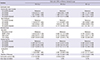
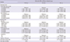
Tables 3 and 4 provide results of multilevel logistic regression for male and female by age. In both male and female, living alone was not significantly associated with depressive symptom in younger adults, while it was significant in mid-aged and older adults. In particular, males were almost twice as likely as females to have depressive symptom in mid-aged and older adults when they lived alone.
The prevalence of depressive symptom according to community income in each family income level
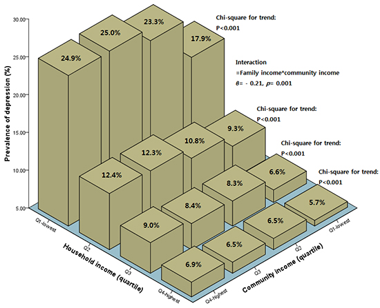
Fig. 1 provides the prevalence of depressive symptom for individuals grouped by family income level according to the community mean income level of their residence. As a result of chi-square test for trend, the pattern with regard to community income level was consistent. The prevalence increased consistently with increased community income level in all groups of the family income (P<0.001), but the magnitude of the difference in prevalence between those with the lowest income and those with highest income was quite different. The gap of the prevalence within the lowest family income group was around 7% (from 17.9% to 24.9%) whereas the gap within highest family income group was around 1% (from 5.7% to 6.9%). It showed that those with lower income are more sensitive to community income level than those with higher family income.
DISCUSSION
The objective of this study was to explore the relationships between individual factors, socioeconomic contextual factors and depressive symptom among Korean population. Previous studies have reported mixed results regarding the effect of average income in a community-level on depressive symptom, while confirming consistent effects of household income on an individuals' depressive symptom (19, 20, 21, 22). Present study shows that increased community income was associated with an increased risk of having depressive symptom. This result has a thread of connection with the recent Korean report which stated depressive symptom, in general, occurs more frequently in high income regions in Korea (27), and it seems that people who live in high income regions are more likely to have depressive symptom due to various contextual stressors such as relative poverty and high competition (28, 29).
Interestingly, our result showed that despite having an equal individual income, the risk of depressive symptom increased continuously from the lowest to the highest regional income level. Moreover a significant interaction between household income and community mean income was found. According to the conditions-cognitions-emotions (CCE) theory, subjective deprivation is the cognitive link between the social environment and mental disorders such as depressive symptom (30). Therefore, it seems that subjective deprivation due to perceived relative income gap plays a key role for increasing depressive symptom. Consequently, an individual who has a higher difference in relative income level may feel more alienation, and this effect seems to be more specific to low individual income groups.
This study found no relationship between income inequality, as defined by the Gini coefficient, and depressive symptom. Previous income inequality studies on depressive symptom have produced less consistent findings (21, 22, 25, 31). A recent review also mentioned such controversial results, suggesting that income inequalities in depressive symptom should be further examined (18). In this study, the proportion of the variance explained by the Gini coefficient was 7.5% whereas it was 19.1% by the community mean income, the Gini coefficient might not have great effect on depressive symptom directly. Similarly, some studies from economics have reported that the Gini coefficient may not reflect a status of inequality properly when the poorest groups are included (32, 33).
Present study showed that female sex was associated with increased risk of depressive symptom. This result is consistent with previous international and Korean studies that showed females were more likely to have depressive symptom than males due to their biological characteristics. And this can be explained by the accompanying loss of estrogens, menopause, the hypothalamic-pituitary-adrenal (HPA) axis and increased functional impairments, psychological attributes affecting vulnerability to life events, and sociocultural roles including a higher burden surrounding childbirth and child-raising duties (3, 8, 9, 10, 11, 15).
As for age, we found that depressive symptom appears to be more frequent among older adults than younger or middle-aged adults (Table 1). In contrast, the odds of having depressive symptom decreased as adults grew older after adjusting other variables (Table 2). Previous studies, including Korean studies, have reported mixed results regarding age. And they suggested that risk of depressive symptom is not influenced by aging independently but other risk factors associated with aging, such as poor physical health including illnesses or lower SES level were more important factors related to risk of depressive symptom (12, 13, 14, 15). This study supports recent Korean studies which have reported that younger adults were more likely to have depressive symptom due to circumstances they face, such as much higher unemployment rate and fierce competition life compared with older adults (3, 11).
With regard to individual SES, depressive symptom was inversely associated with SES as defined by income and educational attainment in this study. This is consistent with the fact that people with lower SES are more likely to have depressive symptom, like many other medical conditions, due to their less favorable access to health care, poorer coping styles, stress exposure, and weaker social support (16, 17, 18). Until recently, only a few Korean studies have included variables of SES and reported that lower educational level and monthly income were associated with an increasing risk of depressive symptom (3, 23).
With regard to the number of having illnesses, this study showed that having more illnesses was associated with increased risk of depressive symptom. There is a great deal of evidence including Korean studies for increasing risk of depressive symptom as physical illnesses increase (15, 34).
In this study, living alone appears to have a higher risk of depressive symptom than living with someone. This finding is consistent with previous studies which have reported those live alone have less social capital which, in turn, is a risk for mental health (35, 36). In other words living alone has a detrimental effect on depressive symptom whereas living with other people could offer emotional support and feelings of social integration. Furthermore, the influence of living alone was stronger on male than female in mid-aged and older adults. It is consistent with a previous study which investigated the effects of living alone on depressive symptom (29). This can be explained by the fact that sex differences in depressive symptom, usually higher in women, were not found in those living alone, and studies which included only women in their sample found no relationship between living alone and depressive symptom (37). Also, it can be interpreted through the facts that the loss of a spouse is more influential to males than females, and males are more dependent on their spouse emotionally (38).
This study has the following limitations. First, given its cross-sectional study design, this study can determine the association among variables and depressive symptom but may not be able to fully explain the causal relationship among them. Further longitudinal and prospective studies are needed to confirm the causation. Second, variables that reflect social infrastructure such as service availability, e.g. the number of psychiatric facility or doctor, which might have an influence on the regional prevalence of depressive symptom, were not included. So, it is suggested that such kinds of variables should be included in further studies. Third, the data was derived from Korean population. As mentioned above, Korea has unique characteristics of socioeconomic contexts from other advanced nations. So, our results cannot be generalized to other nations, and cautious interpretation should be needed.
In spite of these limitations, our study is meaningful in that it is the first to date which explores the relationship between ecological socioeconomic effects, such as community income level and income inequality, and depressive symptom among the Korean population. We found that individual SES is positively correlated with depressive symptom; level of community income has a negative association; those with lower income are more sensitive to community income level than those with higher income; and community income inequality has no detectable relationship with depressive symptom in the Korean population. Interestingly, in the all community income level, those with lowest income had always higher prevalence than those with highest income. Furthermore, despite having an equal individual income, the risk of depressive symptom increased continuously from the lowest to the highest community income level. These findings can provide valuable evidence not only to manage depressive symptom but also to make policy for prevention.
 XML Download