

 PDF
PDF ePub
ePub Citation
 Print
Print


INTRODUCTION
Magnetic resonance electric property tomography (MREPT) was recently re-introduced to noninvasively image the distribution of electric property in human body at Larmor frequency (1, 2). Electric conductivity has been proposed to be used in diagnostic applications (3, 4, 5, 6) and for specific absorption rate (SAR) calculation (7). Over homogeneous regions, the relationship between the electric properties and magnetic fields can be simplified as a Helmholtz equation of the radiofrequency (RF) transmit field, B1+. In MREPT, the electrical properties distribution can be reconstructed from B1+ field information by using the Helmholtz equation. The B1+ magnitude and phase information is acquired separately using different sequences. For example, B1+ magnitude mapping techniques such as actual flip angle imaging (AFI) (8), multiple TR B1/T1 mapping (MTM) (9), double angle method (DAM) (10) and Bloch-Siegert method (11) have been proposed and B1+ phase map has been generally measured using half the phase acquired by a spin echo (2) or multi-echo gradient echo sequence (12) under the assumption that the B1+ transmit and receive phases are identical. In addition, conductivity reconstruction using only the B1+ phase has been introduced (13) and widely used (14, 15), however it can provide accurate conductivity values under the assumption that the spatial variation of B1+ magnitude is negligible. For all these applications and measurements, the conductivity value is needed to be estimated under an acceptable error level.
In MREPT reconstruction process, systemic and statistic error exists. First, systemic error occurs due to invalidity of the spatial homogeneity assumption and of the assumption of equality between B1+ phase (θ1+) and B1- phase (θ1+). When using the Helmholtz equation, boundary artifact is presented at tissue boundaries because of the invalidity of the spatial homogeneity assumption. In a previous study (16), rigorous mathematical error analysis about the boundary artifact was performed and numerical equation which takes into account the inhomogeneity was derived from time-harmonic Maxwell equation. Also, the half value of measured phase,  , is assumed as the B1+ phase due to the assumption regarding the equality of phase. However, as the main field (B0) increases, assumption about the phase equality becomes weaker and reconstructed conductivity map becomes inhomogeneous even over homogeneous regions (17). In the case of B1+ phase based conductivity reconstruction, an additional systemic error occurs inside the object due to the nonnegligible B1+ magnitude variation.
, is assumed as the B1+ phase due to the assumption regarding the equality of phase. However, as the main field (B0) increases, assumption about the phase equality becomes weaker and reconstructed conductivity map becomes inhomogeneous even over homogeneous regions (17). In the case of B1+ phase based conductivity reconstruction, an additional systemic error occurs inside the object due to the nonnegligible B1+ magnitude variation.The second error occurs due to the statistical noise in the B1+ map acquired. This statistic error is a fundamental limiting factor for application of quantitative conductivity mapping because the Laplacian operator, a secondary spatial derivative on the Euclidean space, used in the Helmholtz equation amplifies the statistical noise in the B1+ map. To overcome these limitations, filtering, fitting and integral techniques are applied for conductivity imaging process (2, 13, 14). However, analysis about quantitative error due to noise in B1+ map has not been performed prior to the application of these mentioned techniques. Therefore, in this study, quantitative conductivity estimation error due to the presence of statistical noise in the B1+ map is analyzed and the factors that affect the variation of conductivity estimation inside tissue are examined. In addition, a numerical monomial form is suggested as approximate model for quantitative conductivity estimation error. The results of this study can be utilized for optimal filter design, comparison among reconstruction methods and examination of validity in clinical applications.
MATERIALS AND METHODS
Simulation model and Conductivity estimation method
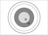
Noiseless B1+ field distribution of radio frequency (RF) transmit field at Larmor frequency was calculated using the Bessel boundary matching (BBM) method (18) which is a very fast electromagnetic (EM) simulation method for simple segmented models. The BBM method was implemented in MATLAB (The Mathworks, Inc., Natick, MA, USA). The numerical simulation phantom shown in Fig. 1 was an infinitely long cylinder placed at the iso-center of a 32 rod quadrature coil and the locations of the RF shield and RF coil were fixed at radius of 45 cm and 16.5 cm, respectively. The simulated phantom's radius, conductivity, permittivity and Larmor frequency was fixed to 5.5 cm, 1.0 S/m, 80ε0, and 128 MHz, respectively, unless otherwise mentioned. The phantom was assumed to be surrounded by a different material having radius of 11 cm. The resolution of the generated B1+ map was 1 mm by 1 mm.
Conductivity σ(r) was evaluated using the Helmholtz equation of Eq. 1 which can be induced from Maxwell's equation. The Laplacian operator was calculated using the surrounding four pixels in the discrete image domain. In addition, conductivity reconstruction using only the phase information was performed using Eq. 2 which is the 2D formation of B1+ phase based method at a single point (13).
Quantitative Conductivity Estimation Error Analysis
To investigate the relationship between quantitative conductivity estimation error and statistical noise in the B1+ map, Gaussian noise was added to the B1+ map prior to MREPT processing. In reality, it is necessary to separately consider the noise in the B1+ magnitude and phase maps due to the separate acquisition of these maps. Statistical noise in B1+ phase map shows Gaussian distribution for SNR >> 1 (19) but, statistical noise in B1+ magnitude map shows diverse distribution depending on the B1+ mapping method (20). However, in this simulation study, the noise in B1+ magnitude map was assumed to be Gaussian distributed which seems reasonable since we focus on quantitative conductivity estimation error not to pattern of the error. Quantitative conductivity estimation error was defined in terms of the normalized root mean square error (NRMSE) obtainable from Eq. 4 with the real conductivity value σreal evaluated using N trials of Monte Carlo simulations. However, in the case of B1+ phase based conductivity reconstruction, reconstructed conductivity value inside homogeneous regions includes systemic error. So, to consider only the effect of statistical noise, the systemic error was disregarded in this case.
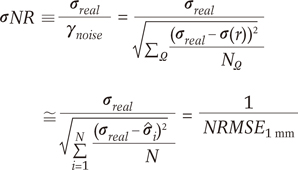
A conductivity-to-noise ratio (σNR) is defined which is the real conductivity value divided by the standard deviation γnoise of the statistical noise in the conductivity map (Eq. 5). In the case of a 1 mm radius object which is identical to the simulated image spatial resolution, since the homogeneous region excluding the boundary is just one pixel, the standard deviation γnoise is equal to the root mean square error (RMSE). Then the σNR is equal to 1/NRMSE1 mm, where NRMSERmm represents NRMSE value over a target tissue of R millimeter radius. Although, the σNR can vary according to size and location of the target object, a previous study (13) showed the spatial dependency of conductivity evaluation error to be marginal. Here we can regard 1/NRMSE1 mm as the general σNR over an object since the resolution of the simulated B1+ map is 1 mm. Thus we refer to NRMSE1 mm as the standard NRMSE.
(Simulation Variable A) Magnitude and phase noise
As referred in the introduction, SNR of B1+ map is one of dominant factors for the accurate estimation of conductivity. In MR scanner, the B1+ magnitude and phase are measured separately using different sequences, and thus the accuracy of B1+ magnitude and the accuracy of B1+ phase are different. In this work, the effect of complex noise in B1+ map on conductivity estimation was investigated. Additionally, to investigate the dependency of conductivity estimation due to noise in separately acquired B1+ magnitude and phase maps, the estimation error due to B1+ magnitude noise or phase noise was calculated individually. To evaluate the accuracy of conductivity estimates with noisy B1+ maps, we performed EM simulations to obtain noiseless B1+ maps. Then, we considered four different cases of noisy B1+ maps generated by adding Gaussian noises.
Noisy B1+ complex - adding complex Gaussian noise to B1+ complex.
Noisy B1+ magnitude and noiseless B1+ phase - adding real Gaussian noise to B1+ magnitude.
Noiseless B1+ magnitude and noisy B1+ phase - argument of noisy B1+ complex.
Noisy B1+ magnitude and noisy B1+ phase (fixed noise level) - combining noisy B1+ magnitude (case 2) and noisy B1+ phase (case 3) using Euler's formula
Specifically, for B1+ complex and B1+ magnitude, the NRMSE of conductivity estimates was evaluated by varying the SNR of B1+. The SNR of B1+ complex and magnitude map can be defined as the average intensity of B1+ inside the region of interest over the standard deviation of noise. However, for B1+ phase, the above definition of SNR was not used directly since the phase itself is not absolute, but phase synchronization at an interval of 2π. The standard deviation of phase noise is a reciprocal of SNR in MR images (19). Thus, for B1+ phase, the NRMSE of conductivity estimates was evaluated by varying the SNR of MR images.
In addition, to investigate the specific effect of statistical noise in B1+ magnitude on conductivity estimation, the NRMSE of conductivity estimates was evaluated by varying the SNR of B1+ magnitude according to conductivity value and B1+ phase with fixed noise level.
(Simulation Variable B) Tissue characteristic & Larmor frequency
The effect of tissue related variables on conductivity estimation was examined. There are many variables associated with tissue, but, in this simulation, only three variables which cause change to the transmit field distribution were dealt with. In addition, the NRMSE value was calculated from conductivity estimates simulated from B1+ maps using human tissue conductivity values previously reported from an ex-vivo study (21). These were done for different frequency values. The specific methods are mentioned below.
1. Surrounding tissue conductivity
The NRMSE from the tissue of interest (Ω), which was surrounded by another tissue (Ψ) at a radius of 11 cm (Fig. 1), was calculated. To examine the effect of the surrounding tissue on the reconstructed conductivity, the SNR level of the B1+ map inside the tissue of interest was fixed to 100 and the conductivity of the surrounding tissue (σout) was increased.
2. Larmor frequency
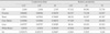
Electric property of human tissues depends on frequency. Therefore, it will vary with the Larmor frequency of main magnetic field, f. Using electric property values from previous study (21) (Table 1), the NRMSE was calculated for seven different tissue types at three Larmor frequencies, 64 MHz, 128 MHz and 300 MHz. Fat, white matter (WM), gray matter (GM), prostate, cerebrospinal fluid (CSF), heart and liver were selected for the simulations. Here, these human tissues were modeled as cylindrical shapes with fixed radius of 5 mm (Fig. 1).
3. Tissue size
This simulation was performed using different sizes of simulation phantom whose radius was altered from 1 mm to 10 mm. Over a homogeneous conductivity region, the conductivity map obtained from the aforementioned MREPT process was averaged to estimate the conductivity value. The number of pixels being averaged (NA) used in the conductivity estimation, is approximately proportional to the area of the phantom. Therefore, NA equal 1, 5, 13, 49, 253 for phantom of radius 1 mm, 2 mm, 3 mm, 5 mm, 10 mm, respectively.
Parametric Modeling of the error in the conductivity estimate
The relationships between the error in the conductivity estimates and other imaging parameters were investigated. The imaging parameters considered here are NA, SNR of B1+, f, σreal σout. For each imaging parameter, x, we modeled that the estimation error, NRMSE, is inversely proportional to a power p of x (Eq. 6).
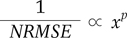
To determine the power of the variable, p, the logarithm of the estimation error was fitted to a linear line of χ and p was determined from the slope of the fitted line. To confirm the fitting accuracy, the R2 (determinant coefficient) value was calculated.
Experimental study
To verify the simulation results, a cylindrical phantom (radius = 5.5 cm and height = 18 cm) was built and imaged. The phantom was filled with a mixture of 0.5% NaCl and 0.5% agar gel. The phantom conductivity measured with a conductivity meter (HI8733N, Hanna Instruments) was 0.82 S/m at 26℃. The measured conductivity value can be used to the conductivity value at 3T MRI because, in the case of saline water, the electric conductivity value is independent of frequency (22). To measure the B1+ magnitude, double angle method (DAM) acquired with 60° - 180° and 120° - 180° flip angle acquisitions was used (10). For B1+ phase measurement, the half value of the phase of a turbo spin echo (TSE) sequence was used. The imaging parameters were as follows: TRTSE/TETSE = 800/20 ms, TRDAM/TEDAM = 2500/20 ms, FOV = 128 × 128 mm2, resolution = 1.0 × 1.0 mm2, slice thickness = 4 mm, 9 slices, and single channel quadrature transmit/receive coil was used. The SNR of B1+ magnitude map was calculated using the law of error propagation similar to the approach in (9) and gave a value of 48. In the case of TSE for B1+ phase measurement; acquisitions were repeated to gather 40 data sets, each 10 data sets were separately averaged to make the SNR vary from 80 to 220. All experiments were performed on a 3T Trio TIM system (Siemens Medical Solutions, Erlangen, Germany). The results were compared using the same size phantom with same SNR variation as the simulations.
RESULTS
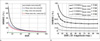
The comparison of conductivity estimation due to three types of noise-magnitude, phase and complex noise type-is illustrated in Fig. 2 to evaluate which error component is most influential. It seems that the magnitude noise in B1+ rarely affects to the conductivity estimation (less than 5% error) according to the green-dot line in Fig. 2a. However, conductivity estimation is sensitive to complex and phase noise as shown in the blue-dash and black-solid line. Hence, it can be interpreted that the phase information is dominant for general conductivity reconstruction method which is in agreement with previous study (13).
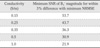
When SNR varies from 10 to 40, the effect of complex noise which contains magnitude and phase noise is more influential than the effect of only phase noise (Fig. 2a). Thus, it can be interpreted that sensitivity of conductivity estimation to magnitude noise increases as SNR decreases in the B1+ magnitude. In detail, Fig. 2b shows the NRMSE curves with fixed phase noise level converge to each minimum NRMSE values as conductivity changes. This convergence means that it is not necessary to increase magnitude SNR more than a specific conductivity-dependent level. In this study, we defined the minimum required B1+ magnitude level that makes the NRMSE to be within 3% difference with minimum NRMSE. This resulted in a value of 61.6, 39.8, 24.5 for conductivity values of 0.1, 0.3, 0.8 S/m. These values were further investigated for conductivity commonly found in in vivo at 3T and were summarized in Table 2. Note that these values are independent of phase noise level (Fig. 2b). Using the p-th degree parametric model, the proportionality relationship between 1/NRMSE and SNR of complex B1+ map (SNRB1+) was fitted to first degree (p=1) as in Eq. 7 with 0.9559 R2 value.
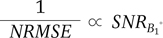
As shown in Fig. 2a, the graphs of conductivity estimation errors due to B1+ phase and complex noise show comparable NRMSE value when each SNR is higher than about 40. Therefore, SNR of the B1+ map in Eq. 7 can be regarded as the SNR of the acquired image for B1+ phase mapping.
The red dashed line in Fig. 2a shows conductivity estimation error when using phase based method. The error graph shows conductivity reconstruction using phase based method is less sensitive to statistical noise in B1+ phase map than using both B1+ magnitude and phase information. However, conductivity reconstruction using phase based method contains additional systemic error since it neglects variation of B1+ magnitude. When phase based method was used for cylindrical object with the radius of 5.5 cm, conductivity value was 20% overestimated as an additional systemic error.
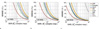
Fig. 3 shows the error in the conductivity estimates for seven types of tissues with the fixed radius of 5 mm for different Larmor frequencies. In general, the accuracy of conductivity estimation increases along Larmor frequency under fixed SNR. This phenomenon can be explained by the fluctuation of B1+ magnitude and phase distribution (23, 24) which increases with Larmor frequency and makes the estimated conductivity value immune against amplified noise in the Laplacian operator. Also, the accuracy of conductivity estimates increases as tissue conductivity increases. Therefore, these two factors, Larmor frequency and conductivity value, can be represented to be directly proportional to 1/NRMSE value (Eq. 8).
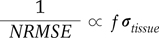
The fitting of the above results gave a R2 value of 0.996 and 0.9999 for B0 and σ of tissue respectively. In calculating the fitting degree for Larmor frequency, the dependence of tissue conductivity on frequency was taken into account. As an example, if the conductivity is estimated using Eq. 1 at 128 MHz, the minimum radius of the homogeneous region required for NRMSE to be less than 10% given a single slice of B1+ map with a spatial resolution of 1 mm and the SNR of 100, are about 128 mm (WM), 99 mm (Liver), 90 mm (GM), 73.8 (Heart), 64.5 mm (Prostate), 33.4 mm (CSF).
To assess the influence of the presence of conductivity material at the outer tissue, the results of evaluated NRMSE with various conductivity values at the outer tissue is seen in Fig. 4a. As seen, the conductivity of the outer tissue has no effect on conductivity estimation of the inner tissue for fixed SNR at the region of interest. As a result, the power of simulation variable σout can be estimated to 0 thus the term which related to σout can be removed.
Fig. 4b shows the relationship between the conductivity estimation error and radius of the tissue. As the radius of the estimation region increases, NA increases. As a result, the conductivity estimation error gradually decreases. More specifically, the NRMSE ratio between 1 mm radius and the others can be found to be  . This ratio is inversely proportional to the NA to a degree of 2/3 (0.9992 of R2 value, Fig. 4c. Since NA is almost proportional to square of the radius, the NRMSE for a Rmm object is related to the standard NRMSE1 mm as the following: .
. This ratio is inversely proportional to the NA to a degree of 2/3 (0.9992 of R2 value, Fig. 4c. Since NA is almost proportional to square of the radius, the NRMSE for a Rmm object is related to the standard NRMSE1 mm as the following: .
The conductivity estimation process is analogous to a kind of filtering process since the homogeneous region with radius Rmm is averaged to estimate σ and NRMSE. Thus, 1/NRMSERmm of estimated conductivity value can be the σNR after filtering.
In summary, quantitative conductivity estimation error due to statistical noise can be represented as in Eq. 10. In addition, the conductivity-to-noise-ratio averaged over an Rmm radius (σNRRmm) can be defined as in Eq. 11.
The unit for frequency (f) is in MHz and σtissue is in S/m. Here, the proportional constant K is added, which directly relates to the σNR and the parameters considered. In our simulation model, the value of K was approximately 640,000. However, this value will depend on many factors such as object shape and location, coil size, etc. The SNRB1+ can be influenced by the B0 value. Here, we assumed that the parameters SNRB1+ and B0 value are independent.
In MREPT, given a fixed Larmor frequency and the conductivity value of target tissue (σtissue), the dependent parameters are SNRB1+ and the number of being averaged pixels (NA). Therefore, the principle of Eq. 11 can be utilized for conductivity mapping. As an example, if we consider a malignant liver tissue of 1 mm object whose conductivity value is 0.66 S/m (at 100 MHz, (3)) and a conductivity map with σNR = 2 is required, the SNRB1+ needed has to be approximately 19,000. In reality, to overcome the lack of SNR, a 22 mm radius homogeneous region is required to estimate the conductivity value with σNRRmm = 2 using a 100 SNRB1+. Therefore, when the conductivity of target tissue, maximum available SNRB1+ and B0 field of the MRI scanner is fixed, the minimum size of detectable tissue using the MREPT process with an averaging filter is determined.
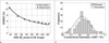
Finally, the principles obtained from the simulation results were compared to experiment study (Fig. 5). According to Table 2, the SNR of the acquired B1+ magnitude map of 48 was sufficient to minimize NRMSE value for a phantom with conductivity value of 0.82 S/m. Thus, the NRMSE value was calculated according to the SNR of the image used for acquiring B1+ phase map (Fig. 5a). The error graphs obtained from simulation and experiment show similar results. Note that the experiment results contain systemic error due to invalidity of the assumption of equality between θ1+ and θ1-. However, the effect of this systemic error was insignificant for conductivity estimation because of the spatially symmetric pattern of this error which vanishes by averaging process (17). Figure 5b shows the histogram of estimated conductivity values which shows similarity between the distribution of conductivity estimation value for simulation and experiment result.
DISCUSSION
Reconstruction of conductivity image using MREPT process suffers from systemic and statistic error. Especially, statistical noise in B1+ map restricts the feasibility of MREPT. Hence, in this study, the relationship between quantitative conductivity estimation error and the parameters that affect the MREPT process was investigated and modeled as in Eq. 11. The systemic constant K can be different value according to the shape of tissue and transmit, receive coil, but the general tendency shown in this study holds.
For quantitative conductivity imaging, SNRB1+ is the most dominant factor because the Larmor frequency and conductivity of target tissue are almost uncontrollable factors. Thus, in the step of B1+ map acquisition, sufficient SNRB1+ have to be guaranteed. Also, SNR of B1+ magnitude and phase map have to be considered separately because the phase and magnitude of the RF transmit field, B1+, is generally acquired using different sequences. In the case of B1+ magnitude map, the minimum required SNR of B1+ magnitude for maximizing the SNR of conductivity map depends on the conductivity value according to Table 2. The minimum required SNR may change according to B1+ magnitude mapping method due to the different distribution of noise in B1+ magnitude map method however it will not vary significantly from the values in Table 2. Therefore, the acquisition time of B1+ magnitude map should be fixed to a minimum to achieve the SNR required and the additional scan time can be used for achieving higher SNR of the acquired image for B1+ phase mapping.
To overcome the sensitivity to statistical noise in B1+ map, a filter was applied to the conductivity reconstruction process (2). In this study, the conductivity estimation process using the average of the reconstructed conductivity value inside a homogeneous region roughly shows the effect of filtering. From statistics, there is an SNR improvement when N number of pixels with independent random noise from a homogeneous region is averaged. However, in MREPT, there is an additional SNR improvement (N2/3 in Eq. [9]) because the Laplacian operator can be regarded as an average over several pixels, i.e., the center and the surrounding pixels. Note that the minimum size of a detectable target tissue is regulated according to the filter size.
Higher Larmor frequency value also reduces conductivity reconstruction error because, as mentioned, the increase of Larmor frequency yields rapid spatial variation of B1+ phase inside the object (24). However, in case of high B0 such as 7T, the assumption about the equality of θ1+ and θ1- is broken and this results in the increment of systemic error. Hence, in using B1+ map acquired at high field MRI scanners, the detection and correction of systemic errors in conductivity map is required.
Through all these relationships, quantitative conductivity estimation error due to statistical noise in B1+ map can be modeled as in Eq. 11. The equation can be used to find necessary SNRB1+ and filter size according to the required conductivity differences between, for example, normal and malignant tissue with a certain size. In addition, using this method, further issues regarding filtering and reconstruction algorithms can be investigated for MREPT.
 XML Download