

 PDF
PDF Citation
 Print
Print


INTRODUCTION
The first article of the Korean Industrial Accident Compensation Insurance Act states that its purpose is for injured workers to return to society, as well as to compensate workers and facilitate their rehabilitation.1 Since return-to-original-work (RTOW) is considered the most desirable for injured workers in return to society,2 the Korean government has set as a policy goal to support individuals returning to original work. Previous studies of return-to-work (RTW) have identified factors related to this outcome, including sex, age, company characteristics, working period, injury type, period for medical care,3 average wage, disability grade, job group (manual worker or not), company size,4 education, consultation experience,5 comorbidities,6 and socio-economic status.7 A systematic review8 concluded that these factors affect RTW after musculoskeletal injury, and another study9 reported that self-efficacy also plays a role in RTW. Since complex factors have been demonstrated as predictors of RTW, it is difficult to use all of these factors practically.
Previous studies have aimed to identify meaningful factors using several statistical methods, e.g., multivariate logistic regression (MLR) has been widely used as a methodological standard in medicine.10 However, machine learning techniques are currently in practice in medical sciences especially for problems on prediction. A problem on prediction is a type of classification problem that can be solved with machine learning techniques. Additional machine learning techniques are becoming widely used, some of which have demonstrated better predictive ability on certain classification problems.1112
This study aims to establish prediction models of RTOW and comparing each model and to apply machine learning techniques to identify factors related to RTOW. By comparing the characteristics of the predictive models, a simple and/or accurate model is identified. This analysis, coupled with a discussion of the advantages and disadvantages of machine learning models, is expected to help establish policy on industrial accidents.
METHODS
Study participants
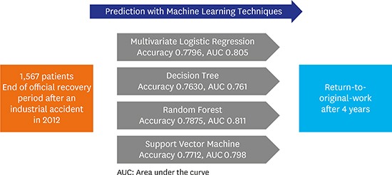
We used data from the fourth Panel Study of Worker's Compensation Insurance (PSWCI), a panel survey conducted by the Korea Workers' Compensation and Welfare Service (KCOMWEL). The nationwide survey sampled 2,000 of 89,921 patients who completed their recovery period in 2012 after an industrial accident. Patients were sampled by the Bellwether method after stratification according to specific variables. The detailed PSWCI sampling methodology is described elsewhere.13 All sampled participants were followed up annually, and the fourth wave of PSWCI data was collected in 2016, four years after termination of the official recovery period.
In the fourth survey, 1,660 patients were followed up successfully, yielding a follow-up rate of 83%. Patients with disability grade 1–3 (n = 25) or 4–7 (n = 68) were excluded from our analysis since high disability grade has been shown to be a strong predictive factor for failure of RTW.3 Moreover, job demand in these patients could be different from that in other patients without a high disability grade, since patients with disability grade 1–7 can receive a monthly pension. Therefore, we analyzed data from 1,567 patients.
Baseline characteristics
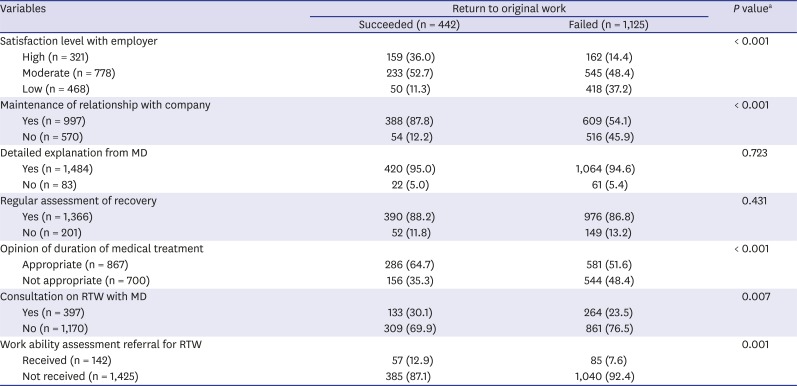
Among the individual characteristics examined, age, education level, earned income, and self-efficacy showed an association with RTOW (Table 1). Alcohol consumption showed a significant P value; however, no trend was observed. All occupational and supportive variables, with the exceptions of ‘detailed explanation from medical doctors’ and ‘regular assessment of recovery,’ showed a significant association with RTOW (Tables 2 and 3).
Table 1
Individual variables (demographical characteristics) related to return-to-original-work of the total dataset (n = 1,567) and χ2 test
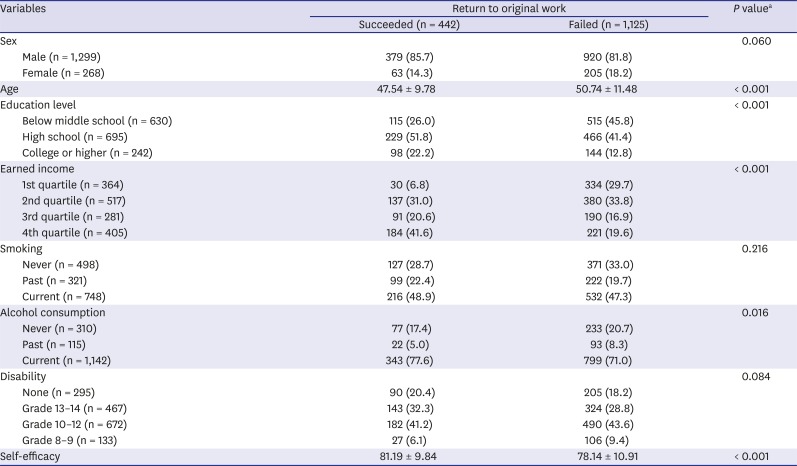
Table 2
Occupational variables related to return-to-original-work of the total dataset (n = 1,567) and χ2 test
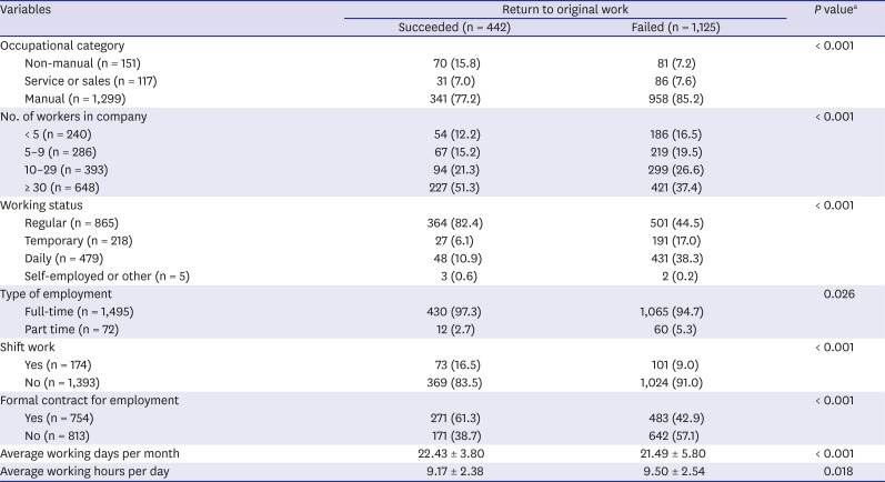
Table 3
Supportive variables related to return-to-original-work of the total dataset (n = 1,567) and χ2 test
Methods
The total dataset was randomly divided into two subsets, a training dataset (75%, n = 1,175) to make prediction models and a test dataset (25%, n = 392) to report the prediction ability of each model. The random selection was done by the function ‘sample’ of R with setting seed numbers in order to assure reproducibility. The dependent variable in our analysis was working status at four years after termination of the official recovery period in 2012. The independent variables examined are listed in Tables 1-3; χ2 tests were performed for each variable. A detailed description of the questionnaire variables from PSWCI is provided elsewhere.14
Two MLR models were established, one with the total dataset and another with the training dataset. The model with the total dataset was compared with the model from the training dataset, and the odds ratio (OR) from the two models were assessed. ORs from the total model were used to describe the results, while ORs from the training model were used to adjust and optimize the model's predictive ability. In the classical analytic models, P values below 0.05 were considered significant.
Models using machine learning techniques including decision tree (DT),15 random forest (RF),16 and support vector machine (SVM)17 were formed with the training dataset. To assess the predictive ability of each training model, we transformed and reconstructed the models by excluding unimportant variables and/or tuning hyper-parameters to improve the model's performance with automated process using the R package caret (R Foundation, Vienna, Austria).18 Variable importance was assessed by visualizing the varImp function of the package.
The best models with the highest predictive ability for each technique were selected as the representative models. We compared all necessary variables and the model performances by calculating the accuracy, sensitivity, specificity, kappa value, and area under the curve (AUC). The final predictive values were reported with mean ± standard deviation from 10 iterations of the same procedure after random allocation of training/test datasets with different seed numbers.
RESULTS
MLR analysis
Although many variables showed a statistically significant association with RTOW by the χ2 test, only six factors showed significant ORs in the MLR models. A potential explanation for this finding is that some variables might confound other variables. The trends were very similar between the total model and the training model. Moreover, all significant factors in the total model also showed significance in the training model (Table 4).
Table 4
Logistic regression analysis for return-to-original-work using the total and/or training model
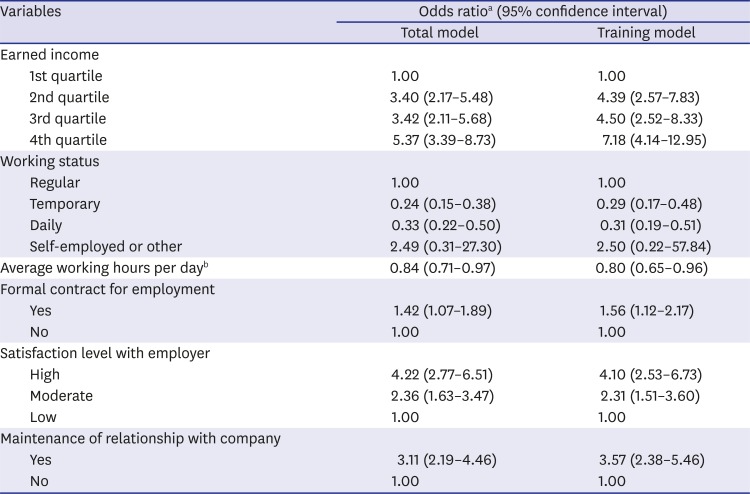
aAdjusted for sex, age, education level, smoking, alcohol consumption, disability, self-efficacy, occupational category, number of workers in company, type of employment, shift work, average working days per month, detailed explanation from a medical doctor, regular assessment of recovery, opinion of duration of medical treatment, consultation for return-to-work with a medical doctor, work ability assessment referral for return-to-work, and all variables in this table; bOdds ratio with normalized value.
Earned income was the strongest predictor for RTOW and showed a directly proportional relationship: The greater was an individual's income, the better was the chance that he/she would return to his/her original work. Temporary or daily working status acted as a negative predictor of RTOW. Average hours worked per day showed an OR less than 1.0, meaning that the more hours per day an individual works, the more difficult it is for him/her to return to his/her original work. When a formal contract of employment was present, RTOW was easy. Moreover, when a worker was satisfied with the employer's support during the duration of the official recovery, the worker could return easily. Maintenance of a relationship with the original company also showed a high OR, although this variable potentially has multicollinearity with ‘satisfaction level with employer.’ However, no significant variables were associated with any of the supportive factors from hospitals or KCOMWEL.
We next compared a predictive MLR model using all variables with another model using only the six most important variables (as assessed by ORs) and the varImp function; the former showed better predictive ability.
Inter-technique comparison of machine learning techniques
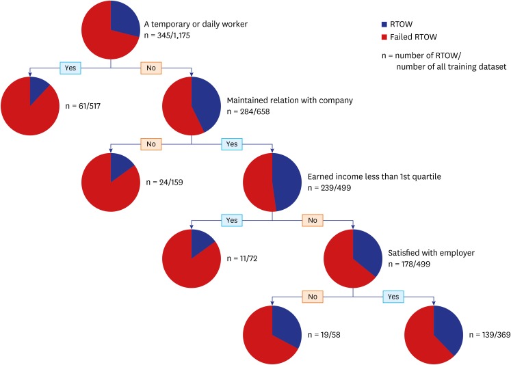
Prediction models with DT, RF, and SVM were established. For a DT model, a pathway was established. Fig. 1 displays a visual depiction of the DT model algorithm. A variable-selected model of RF showed an inferior result to the initial model. The best RF model with the model containing all variables was established via grid search, of which the hyperparameters was the following: 3 nodes, 500 trees and 3 tries.
An initial SVM was established with all the variables included, which yielded the accuracy of 0.7270, however, the very low sensitivity of 0.0273. The importance plot for the SVM showed the order of importance of the variables: the first was working status, and the following variables were earned income, maintenance of relationship with company, and satisfaction level with employer, in order (Supplementary Table 1). We could upgrade the function of SVM by selecting these four variables, which yielded better accuracy and sensitivity (0.7602 and 0.5909). After hyperparameter tuning by grid search algorithm, the final SVM model was established. We showed detailed process of establishing the DT, RF, and SVM model in Supplementary Table 2.
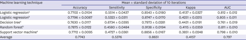
The MLR and RF models showed optimal prediction when they used all variables, while the others showed optimal prediction when they used only the significant variables. Table 5 shows the final performance comparison of the models from each machine learning technique. The RF model showed the best performance in terms of accuracy and specificity (0.7875 and 0.9138, respectively). The DT model showed the highest sensitivity and kappa value (0.6734 and 0.4431, respectively). The MLR model using significant variables showed the best AUC (0.812). Ranked in order of predictive accuracy, the models were: RF, MLR, SVM, and DT. However, the accuracy of the models had only minor variation (maximally 0.025) despite statistical significance (Supplementary Table 3).
Table 5
Performance of machine learning techniques
Supplementary Table 1 lists the factors that were selected finally in relation with RTOW in the MLR, DT, RF, and SVM models. Each model contained four to six significant variables. The DT and SVM models recognized only four variables as significant; the RF model, five; and the MLR model, six. When we analyzed the first random seed, the order of significance of the factors was different in each model. As also reflected by the ORs of the MLR analysis, the MLR model identified earned income as the most important variable, whereas the DT and SVM models identified working status as the most important variable. The RF model identified ‘maintenance or relation with company’ as the most significant variable. This order of significance differed by a new random allocation of training and test dataset. However, the four variables were always on the top of importance in all the models.
DISCUSSION
This study showed that machine learning techniques can predict the probability of RTOW by four years from the end of the official recovery period. The RF model showed the best performance, but the other models showed almost comparable performance. This is the first study using machine learning techniques to predict RTW. Machine learning techniques have a more complex mathematical basis than classical MLR modeling; however, since they do not assume linearity, machine learning models are more flexible and require fewer variables.
Predictive models with machine learning techniques are anticipated to be adopted more frequently in medicine and social sciences in the future. Prediction of various outcomes by machine learning techniques has already become common in medicine, such as mortality,12 surgical outcomes,24 and psychiatric illness.25 This study used similar methodologies of these previous trials: comparing variables with conventional statistical methods, establishing machine learning models with selecting all the variables or selected variables for efficiency, and hyperparameter tuning process to maximize the predictive accuracy.
When optimizing hyperparameters of RF and SVM models, we used the grid search mechanism which is a traditional method with some weaknesses. The grid search does not guarantee that the results were mathematically the most optimal. Therefore, novel methodologies such as random search, Bayesian optimization, gradient-based optimization, and evolutionary optimization are being developed and applied currently. This study did not used these current methods for hyperparameter tuning because of limited software resources of the R package caret. However, although our methodology could not guarantee a mathematical robustness, the grid search mechanism has been widely used, so that we estimate that our results are not far from the very optimized values. We also expect that this simple method could be applied practically in KCOMWEL.
If our models be applied in practice of KCOMWEL, it would be possible making an individual policy of RTW of an injured worker; for example, providing an early reemployment administration service to a worker who is expected to fail of RTOW. However, there might be considerations other than a simple prediction. In this study, we just showed the possibility of prediction and it is necessary more detailed discussion on availability of the prediction.
Comparing all the models introduced in this study, the RF model showed the best performance (Table 5) in terms of accuracy significantly (Supplementary Table 3). However, since this model used all variables in its analysis and its tuning process is automated, and RF sometimes yields unstable results by each trial, its practical applications are limited.
The SVM model showed results that were similar to those of the MLR model, even if they used only four variables in the analyses. This feature of SVM modeling — i.e., better efficiency with fewer variables11 — has potential practical advantages. A modeling method using SVM is referred to as a ‘black box’ model because of its mathematical complexity26; thus, the interpretation is limited.
Classical MLR modeling yields ORs of independent variables that affect dependent variables. The theoretical assumption behind this method is that ORs approximate risk ratios if the sample size is sufficient. However, regarding epidemiology, it is still unknown what is the meaning of features selected in SVM and RF. Future efforts should investigate how to interpret factors identified by other machine learning techniques in the context of social epidemiology.
Even if the accuracy is inferior, the results of the DT model seem to represent an acceptable compromise of practice and interpretation, because the mathematical methodology used to discriminate variables that maximize information gain is simpler than that used in other machine learning techniques. In particular, the DT model in this study showed a one-way path that is very easy to implement in practice. If an employee is not a temporary or daily worker, maintains a relationship with the company during the recovery period, has earnings in the upper quartile, and is satisfied with the employer's convenience, the DT model predicts that he/she will return to his/her original work with a sensitivity and specificity of 67% and 80%, respectively. Therefore, the DT model's four questions could be used when assessing how to best support patients from industrial accidents.
The differences between the techniques were not prominent; only 0.025 of difference of accuracy between the superior model (RF) and the inferior one (DT). These results are similar to a comparison study that showed statistically not significant differences of methodologies with naïve Bayes, RF, DT, SVM, and MLR even though the MLR model showed the best performance.27 It means that there is not so much to expect in choosing the most elaborate method. It is necessary to select an appropriate model by advantages and disadvantages in order to predict a worker's possibility of RTOW. For example, RF model for the best accuracy; DT model for clear and easy-to-use standard; SVM model for a simple composition of necessary variables.
Regarding the characteristics of important predictors for RTOW, all models selected similar variables as important for predicting RTOW, although some differences were observed among the models. Four variables — earned income, maintenance of relation with company, satisfaction level with employer, and working status — were selected in all models. These variables can be classified as ‘variables related to the company itself.’ While nearly all the variables except these important variables were also significantly associated with RTOW in the χ2 analyses, no significant effects were observed for any of the variables in the machine learning models.
This finding means that the strongest component influencing RTOW and its durability is a worker's company. This finding is consistent with a previous study3 that identified workplace characteristics as significant predictive factors for RTW. Another study from the first PSWCI14 reported that sex, age, regular recovery assessment, and opinion of duration of medical treatment were related to RTW, similar to the findings of our study. However, the data obtained from the longer follow-up in our study suggest that company-related factors were more influential than individual or supportive factors.
As well as the four variables, formal contract for employment and average working hours per day were selected in the MLR model and age in the RF model. However, the additional variables were not more significant than the four variables in each model while the four variables showed little differences among the models and internal fluctuations. Therefore, although there were some differences due to technical methods, all models indicated that variables related to the company itself would influence RTOW. In this point, staffs and medical practitioners who are working for patients aiming RTW should consider the characteristics of the patients' original companies.
Earned income showed the biggest ORs in the MLR model and had a positive gradient, as all models selected it as an important variable. This feature should be discussed in the context of social justice, e.g., whether workers' compensation insurance is adequate in the social security system. KCOMWEL provides various services and programs for RTW, as mentioned in the Introduction. Of these services and programs, consultation for RTW with medical doctors and work ability assessment referral for RTW were associated with RTW in the χ2 analysis (Table 3). However, this effect was not observed in the MLR model or in the others. This finding suggests that these services were closely associated with company-related factors, i.e., the services necessary for RTW were provided to workers who already had a good base for RTW. If the services had similar effects on all workers, related factors should have been detected in the machine learning analyses. This result is strongly supported by the segmented labor market in Korea: a worker's situation before injury influences the quality of employment after RTW.28
This study has some limitation. It did not use variable weights, because it is unclear how to handle these weights when developing training models. Weights are used to assure representativeness, but it is unknown how these weights should be used to guide training and test datasets. Moreover, machine learning techniques are not typically used with weighted variables. The follow-up rate was 83%, and this study did not consider dropouts. Therefore, the results of our study are not necessarily applicable to all workers nationwide. However, the results of previous studies and the results of the MLR model without weighted variables in this study were similar.
We showed that, by using only four to six variables at the end of a worker's recovery period, the probability of RTOW can be predicted with an accuracy of 76%–78%. Since additional factors that were not included in our study might change the predictive performance of the models, future studies are needed to investigate and predict RTW more precisely.
 XML Download