

 PDF
PDF ePub
ePub Citation
 Print
Print


ABBREVIATIONS
NONMEM
NONlinear Mixed Effects Model
PK/PD
pharmacokinetic/pharmacodynamic
SE
standard error
EBE
empirical Bayes estimate
MVN
multivariate normal
CL
clearance
PRED
prediction
IPRE or IPRED
individual prediction
MAP
maximum a posteriori
L
laplacian method
LI
laplacian with interaction
FO
first order
FOI
first order with interaction
FOCE
first order conditional estimation
FOCEI
first order conditional estimation with interaction
LL
log-likelihood
NONPAR
nonparametric
THEO
theophylline
PHENO
phenobarbital
MAXEVALS
maximum number of function evaluation
INTRODUCTION
NONMEM® (NONlinear Mixed Effects Model) is the most widely used software for the population pharmacokinetic/pharmacodynamic (PK/PD) modeling and simulation, also is the standard tool for drug development as well as regulatory approval. NONMEM® uses inter-subject variability parameter η to describe the individual differences in PK/PD parameters. However the standard error (SE) of the empirical Bayes estimate (EBE) of the inter-subject variability parameter η is not provided in the NONMEM® output file. The SE of EBE is an enhanced model diagnosis tool to assess the precision of the estimated inter-subject variability parameter η. Also the SE of EBE can be used for simulation considering the uncertainty in the inter-subject variability [1].
The SE of EBE of the inter-subject variability parameter η is not available in the output file of NONMEM®. Therefore postprocessing after a modeling NONMEM run is necessary to obtain the SE of EBE. Writing one's own code requires careful thinking and programming expertise. A Perl based automated utility to calculate the SE of EBE is available in PsN® version 2.2.6 or later [2]. However, a more direct method to obtain the SE of EBE is possible with NONMEM® VI using one of the internal variables, POSTV. Unfortunately, this feature is not available in the previous versions of NONMEM®. The POSTV matrix is not available in the new version of NONMEM® 7, either. However, the elements of the POSTV matrix are available as ETC columns in the .phi file, one of the new output files from NONMEM® 7.
The objectives of this study are to illustrate how to directly obtain the SE of EBE by the use of NONMEM® VI internal matrix POSTV and to evaluate the performance by comparing the results with other methods. The contents of this paper are as follows. In the methods section, theoretical backgrounds for calculation of the EBE and the standard errors of EBE are overviewed along with the descriptions on the four models and the two datasets used to assess the different ways of calculating the standard of errors of EBE. Then detailed explanations on the three methods, including the suggested simple method of obtaining the covariance matrix of EBE in NONMEM® VI using verbatim code, are provided. In the results section, the numerical results are summarized and compared. Lastly, the discussion section concludes with a few remarks and conclusions.
METHODS
The following notations are used for PK/PD modeling using NONMEM®:
F=f1(θ, η, χ): the model predicted (i.e., fitted) value (F), model parameter (θ), interindividual random variability parameter (η), and covariates (χ) defining structural model to explain pharmacokinetics/pharmacodynamics
Y=f2(F, ε): the observation (Y) given by F and the residual (or intra-individual) variability parameter (ε).
η~MVN (0, Ω): inter-individual random variability modeled using multivariate normal (MVN) distribution with mean zero and covariance matrix Ω
ε~MVN (0, Σ): intra-individual (i.e., residual) random variability modeled using multivariate normal distribution with mean zero and covariance matrix Σ
θ, Ω, and Σ are constants while η and ε are random variables. The function f1 represents a structural model describing the relationship between the PK/PD observations and the model parameter θ, while η and ε represent the stochastic model components describing the randomness unexplained by the structural model.
The typical PK/PD of the population is summarized by θ, and individual PK/PD parameters are expressed as a combination of θ and η. For example, systemic clearance is expressed as
CL=θCL·exp(ηCL), Equation 1
where θCL is the typical value and ηCL is the corresponding inter-subject variability following normal distribution with mean zero and covariance, e.g., Ω11. In other words, the typical value of a PK/PD parameter is the value of PK/PD parameter with η=0. F is called the typical predication (PRED) when η=0, and the individual prediction (IPRE or IPRED) when η=η̂ the EBE of individual eta.
In addition to the inter- and intra-subject variability, there can be another level of random variability called inter-occasion variability which describes the random variability among the different treatment occasions, for example, different visits. Implementation of inter-subject and intrasubject variability can be accomplished using the corresponding NONMEM® variance parameters η and ε. However, implementation of inter-occasion variability requires an elaborate coding using the inter-subject variability parameter η, because η now has to match the new variability introduced to model the inter-occasion differences. The developed method of computing standard error (SE) of EBE using NONMEM® VI internal matrix POSTV can be applied to η for inter-subject variability as well as η for inter-occasion variability without further modification of NONMEM® control code.
The random variable η cannot be directly observed but can be estimated using subject level observations (Y, i.e., dependent variable) and the final estimates of θ, Ω, and Σ. The estimates of each subject's η (η̂) has several namesrealized η, post hoc η, empirical Bayes estimate (EBE) of η, or maximum a posteriori (MAP) estimate of η. There are several numerical methods to estimate the aforementioned PK/PD parameters. The available estimation methods from NONMEM® VI and their characteristics are as follows [3]. FO method employs "First Order" linear approximation of F with respect to η. Laplacian method (L) uses "Laplacian" integral approximation of the objective function using up to the second order partial derivatives. FOCE method stands for "First Order Conditional Estimation," for which individual η (η̂) is estimated during the minimization process [3]. Individual η estimates (η̂) are not calculated during the minimization process for the FO method, however they can be estimated with the final θ, Ω, and Σ with the POSTHOC option. In the FOCE or Laplacian method, computation of the individual η estimates (η̂) is necessary during the minimization process. The difference of FOCE objective function with respect to the Laplacian objective function is the use of the first order partial derivatives for the linear approximation whereas the Laplacian method uses up to the second order partial derivatives [4]. The computation time increases in the order of FO, FOCE, and Laplacian. The INTERACTION estimation option considers interaction of η and ε, and uses η̂ instead of 0 for η during the calculation of variance of Y. INTERACTION option does not affect the output for the additive residual error model, but produces different estimates which are regarded as more accurate for other residual error models (proportional error, combined additive and proportional error, power function error, etc.).
When f1 is linear with respect to η, joint objective function is used for estimation of θ, Ω, Σ, and [5]. When f1 is nonlinear with respect to η, NONMEM constructs a separate objective function to estimate EBE in addition to the objective function to estimate θ, Ω, and Σ. Objective function for EBE in NONMEM® as well as ADAPT 5 [6], a similar PK/PD modeling and simulation software, is as follows:
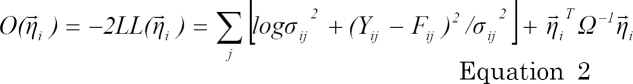
where ij denotes j-th observation of the i-th individual, and LL( ) is the log-likelihood.
) is the log-likelihood.The uncertainty of the estimated θ, Ω, Σ, and η̂ can be obtained by computing the corresponding standard error which is the standard deviation of estimates. However, special consideration is required for η̂ because there is an upper limit for the uncertainty in η̂. Even if there are no data for a particular individual, ω̂ (estimated inter-subject variability for the population data at hand) can be an estimate of the uncertainty about η̂ of this individual, because of the assumption that the individual belongs to the population characterized by ω̂. For this case, individual η shrinkage, the standard error of divided by the corresponding ω̂, could be a better measure of uncertainty [7].
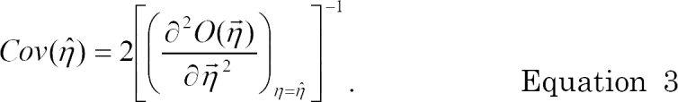
In NONMEM® VI, the standard error of EBE of η̂ can be computed using the following asymptotic expression for covariance of an estimate, assuming that the estimated θ, Ω, and Σ are the true values [5].
The usefulness of EBE of η is manifold. Individual PK/PD parameters and accordingly individual drug concentrations or effects are described using EBE [8-10]. EBE can be used for screening covariates for the structural model development [11]. If relationships between covariates and EBEs do not exist, EBE theoretically should have no trend with the covariates. Apparent relationship between EBE and covariate indicates the necessity of further refining the structural model, for example, including that covariate in the structural model. However, such a method is not recommended when there is difference between the empirical distribution of η̂ and the estimated Ω, i.e., when the shrinkage is greater than about 20%. The empirical distribution of EBE can be used to test the normal distribution assumption on Ω, or the validity of the mixture model, or the necessity of using some other kind of nonparametric distribution. Since EBEs are used in the objective function calculation in FOCE or Laplacian method, both methods rely on accurate EBEs. In NONMEM® VI, EBE can be used as support points to calculate the joint density for NONPAR (nonparametric) estimation option [12].
Two datasets and four population pharmacokinetic models
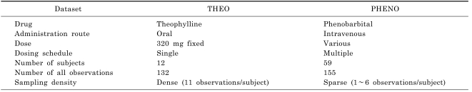
The two datasets in NONMEM® VI distribution media, THEO and PHENO, were used to compare different methods of computing the SE of EBE. These datasets are readily available and the use of these public datasets makes it easy to compare the results of other available methods of the future.
THEO dataset has 132 observations from 12 subjects. There are 11 observations per subject following an oral administration of 320 mg theophylline. Therefore THEO dataset can be regarded as an intensively sampled dataset. PHENO dataset has 155 observations from 59 neonates with multiple intravenous administrations of phenobarbital. There are 1 to 6 observations per subjects, which can be regarded as a sparsely sampled dataset (Table 1).
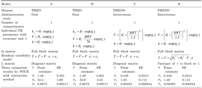
Using the two population datasets, four different PK models were tested for the calculation of the SE of EBE of η. One compartment PK model with variations in the structural part or residual error model was used to fit the test datasets. Models A and B used THEO dataset while Models C and D used PHENO dataset. All of the individual PK parameters were modeled using log-normal distribution as in Equation 1. Models B, C and D had covariate effect on the typical volume of distribution V while Model A had none. All the models had block omega matrix, and used combined proportional and additive residual error model. The four tested models are summarized in Table 2. The model prediction F for each dataset can be calculated as follows.
For THEO dataset (one compartment PK model with oral administration),
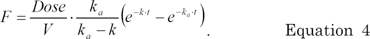
For PHENO dataset (one compartment PK model with intravenous administration),

using the superposition or the convolution of input and disposition function.
Three computation methods for the standard error of EBE
Method 1. User written function in R
To compute the standard error of EBE of η, $PRED routine and objective function routine for EBE (OBETA.FOR in NONMEM® VI) need to be coded. R 2.7.1 and R 2.8.1 for MS-Windows were used as programming tools. Objective function routine for θ, Ω and Σ can also be coded and fitted. However due to the very long computation time, final estimates of θ, Ω and Σ from NONMEM® run were used to estimate EBEs and their standard errors.
The role of $PRED routine in NONMEM® is to calculate F, G and H vectors or matrices. F has different meaning in different estimation methods. F is typical prediction (PRED) in the FO method and individual prediction (IPRED) in the other estimation methods. G is the partial derivative of F with respect to η evaluated at η̂, which is necessary to calculate the total objective function value for θ, Ω and Σ. For the estimation of EBE, G matrix is not necessary because the total objective function value does not have to be calculated. H is the partial derivative of Y with respect to ε, which is necessary for the calculation of σ2ij in the objective function for EBE.
For minimization, "L-BFGS-B" algorithm in 'optim' function was used with zero initial values. Other minimization algorithms in R showed almost the same results with more than three identical digits. The R codes for substitution of $PRED and OBETA.FOR are shown in the appendix. This method uses explicitly equation 3 and it is well-known and described in many textbooks. Therefore we chose this method for the calculation of SE of EBE as a standard one.
Method 2. PsN 2.2.6 or later
PsN is a free software for pre- and post-processing of NONMEM® runs and outputs, developed by the Pharmacometrics Research Group at Uppsala University and available at http://psn.sf.net/. One added feature of the PsN 2.2.6 with respect to the previous versions is the computation of standard errors of EBE of η. The new command for estimating the SE of EBE of η is '-se_of_eta.' To do this, PsN Internally generates modified NONMEM® control stream and dataset for each subject. Parameters θ, Ω and Σ are fixed at the values obtained from the estimation step for all the subjects. ETAs in the original model are replaced with new added THETAs to obtain the standard errors of these added THETA estimates. Modified dataset for each subject has newly appended rows as many as the number of etas, and EBAY (previously TYPE) column to classify the DV types. PsN fits each subject data one by one with MATRIX=R option in $COVARIANCE. Then the standard errors of the added THETAs are the standard errors of the original EBE of η's [13].
Method 3. POSTV matrix within NONMEM® VI
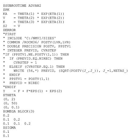
POSTV or ROCM36 is a matrix that is not very well documented in NONMEM® VI User Guide. The only available explanation about ROCM36 in NONMEM help is "individual's posterior variance-covariance matrix." However, the square root of the diagonal elements of POSTV matrix can be used to calculate the SE of EBE of η. Technical difficulty in using POSTV is that the elements are very frequently updated so that if the matrix is printed, the amount will be too bulky. To avoid this problem and obtain one line output per subject, verbatim code must be used. NONMEM® control stream for extracting the diagonal elements of POSTV matrix is shown in Fig. 1.
To print out the POSTV matrix, three new variables have to be defined: PPSTV1, PREVID, and CVRSTEP. PPSTV1 retains the first element of the previous POSTV matrix, and PREVID delivers ID of current record (NIREC) to the next call of $ERROR routine. CVRSTEP is set to 1 during the $COVARIANCE step. The INCLUDE statement is necessary because LVR, defined in SIZES file, is necessary to define the size of the matrix POSTV. The POSTV matrix is available through ROCM36 (presumably 'read only common variable 36'). The contents of the POSTV matrix is updated very frequently even during the computation of θ, Ω and Σ. Change in POSTV(1,1) value for the same subject number (NIREC) indicates that minimization process reached the $COVARIANCE step. To obtain the SE of EBE, the square roots of the diagonal elements of POSTV have to be printed using, for example, file stream 56 (i.e., 'fort.56').
Finally, file stream 56 has to be closed at ICALL=3 step. This is not necessary if extra files are not opened within $TABLE step. However, explicit closing of the open file stream is recommended for safe termination of NONMEM® VI. If $PRED is used instead of PREDPP (ADVAN subroutines), verbatim code has to be placed within the $PRED routine.
Comparison among computation methods
To compare the computed SEs of EBEs among different methods, correlation coefficients were calculated. However, all of the correlation coefficient values were so close to one that small differences were not properly captured in the preliminary analysis. Therefore the percentage of observing 5 percent or greater difference with respect to the result from the theoretical method (Method 1: user written function of Equations 2~5 in R) was employed as the most sensitive way of comparison.
RESULTS
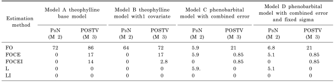
Five estimation methods were tested for each model: FO (First Order), FOCE (First Order Conditional Estimation), FOCEI (First Order Conditional Estimation with Interaction), L (Laplacian), and LI (Laplacian with Interaction). FOI (First Order with Interaction) was explored using Methods 1 & 2, however the result was not used for comparison because POSTV was not available with METHOD= ZERO INTERACTION option. Other estimation options were set at default values except that the maximum number of function evaluation (MAXEVALS) was set at a generous number of 9999. As a measure of comparing the results from the three methods, the frequency of discrepancy in the results greater than 5% compared with the R code result (Method 1) is shown in Table 3. Method 1 is used as reference to compare the degrees of discrepancy of computation results from the other methods, because the R code was straightforwardly implemented equation 3. On the other hand, the detailed computation algorithms of the other two methods are either unavailable to the public or very difficult to track. EBEs and standard errors computed by method 1 are in appendix tables.
There was no discernable difference in the point estimates of EBE of η among all of the three methods, for the various estimation methods and the datasets. The degree of differences in the results from the three computation methods for the SE of EBE of η depended on the employed estimation method. All the three methods produced almost the same results when Laplacian estimation method (L or LI) was used. For the conditional estimation methods (FOCE or FOCEI), there was no noticeable difference between the computed SE estimates from R code (Method 1) and PsN (Method 2). When FOCEI estimation method was used for the sparse sampling dataset of phenobarbital, the percentage occurrence of POSTV method results (Method 3) differing more than 5% compared with R code result (Method 1) was less than 1%. For the extensive sampling dataset of theophylline, greater than 5% difference in EBEs occurs 3% to 17% with FOCEI. The degree of difference got larger for the simple FO estimation. Greater than 5% difference between Method 1 and Method 3 occurred more frequently (21% to 86%) with the FO method.
DISCUSSION
Estimation results are usually provided as predicted mean or typical values for the unknown parameters of the system along with measures of inter-correlation and precision associated with the parameter estimates. Standard errors of the parameters are easy to explain and understand about the precision of the parameters. In population analysis where hierarchical structure (ie, population level and individual level) is involved, investigation of the SE of EBE for individual level can be used as an enhanced model diagnosis tool to assess the precision of the estimated inter-subject variability parameter as well as for simulation considering the uncertainty in the inter-subject variability, in addition to the SE of population parameters.With the availability of SE of EBE during simulation, the discussion about the central tendency or outlying values for individual predicted values can be possible, which can be a useful information for developing indivualized therapy.
Three methods of computing the standard error of empirical Bayes estimate of the inter-subject variability parameter η for NONMEM were explored and the performance was evaluated. The SE of EBE of the inter-subject variability parameter η can be computed in a direct and robust way by using the POSTV matrix in NONMEM® VI without additional postprocessing efforts. The POSTV matrix is not available in other versions of NONMEM®. However the elements of the POSTV matrix are available as ETC columns in the .phi file from the new version of NONMEM® 7. Such SE of EBE from NONMEM® 7 was almost identical with the POSTV from NONMEM® VI. The proposed simple and robust method of computing SE of EBE using POSTV is not reported in the standard NONMEM® output file. The reason might be that there are other methods for computing SE of EBE using uncertainties associated with θ, Ω and Σ together. The computation differences with respect to the result from R code may be due to the fact that R function "optim" uses numerical calculation of gradient and hessian while NONMEM® uses analytical partial derivatives partially for the PK models using ADVAN2 routine. However, when LAPLACIAN is used, NONMEM® also uses numerical methods for gradient and hessian calculation so that the result showed no difference with respect to PsN and R.
There are a few limitations of using POSTV for obtaining SE of EBE. The method assumes no uncertainties for the estimated θ, Ω and Σ, and cannot be used with the METHOD=ZERO INTER estimation option. The discrepancies of the computation results with respect to the other two computation methods were observed, and the differences might be attributed to the analytical versus numerical calculation of derivatives.
PsN is a convenient tool to obtain SE of EBE, however PsN fits modified model to the modified individual datasets. In addition, PsN may produce quite different point estimates of EBE when the EBE values are close to zero. Therefore, computing the point estimate of EBE using individual data should be used with caution. The source of this difference might be due to the different minimization algorithm for EBE computation to the algorithm for the estimation of θ, Ω and Σ. Not much is known about what algorithm is used for computing EBE, whereas quasi-Newton type derivative free algorithm (a variant or modification of derivative free Davidon-Fletcher-Powell algorithm in ZXMIN1. FOR) is used for estimating θ, Ω and Σ.
In conclusion, POSTV matrix can be used for a simple and robust computation of SE of individual ETA values in NONMEM® VI. The results were comparable with other computation methods. The degree of discrepancy was smallest in LI method, smaller in FOCEI than FO.
 XML Download