When a prodrug is administered orally, it undergoes complicate processes of absorption, distribution, metabolism, and excretion. To understand these processes for metabolites, Cummings and Martin published results on the excretion and accrual of drug metabolites in 1963.[4] This provides the basis for the pharmacokinetics of drug and its metabolites and can be readily applied to study the pharmacokinetics of prodrug. Since then, many theoretical analyses and reviews, related to prodrug pharmacokinetics, have been published.[5678910] A thorough understanding of prodrug kinetics is daunting and may be achieved using sophisticated physiologically based pharmacokinetic (PBPK) modeling.[1112]

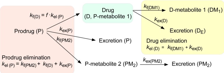
To get some insight pertinent to prodrug kinetics, we consider a simple scheme for the fate of a prodrug (P) after intravenous administration (Fig. 1). A fraction of the prodrug (f) is metabolized and produces a parent drug (D) with a first-order formation rate constant, k_f(D). The drug (D) may be further metabolized to a daughter metabolite (DM₁) or excreted. The elimination rate constant of the parent drug, k_el(D), is expressed by the sum of the formation rate constant of the daughter metabolite, k_f(DM1), and the urinary excretion rate constant, k_ex(D). More than one metabolite may be formed with a formation rate constant, k_f(PM2), and then excreted with a rate constant, k_ex(PM2). Otherwise, a fraction of the drug is excreted into urine as unchanged form (P) with a rate constant, k_ex(P). The overall elimination rate constant of the prodrug, k_el(P), is the sum of k_f(D), k_f(PM2), and k_ex(P). No matter how complex the pathways may appear, the time course for the change of metabolite amount can be described by a general relationship: rate of change of metabolite amount in body = rate of formation − rate of elimination. [56] However, a full mathematical description of this model is still complex and difficult to solve. We will further simplify this model to have clear understanding of the factors influencing the amount of parent drug in the body.

Consider a simple case of a two-step consecutive first-order irreversible reaction:

This model provides the basis for developing more complex models. Thus it is crucial to understand this reaction kinetics thoroughly for further study. Here, we use simple notations for the sake of clarity. We can set up the following three differential equations to describe the change in amounts of A, B, and C over time.

At t = 0, A = A₀ and B = C = 0, and A + B + C = A₀ at all times. The Eq. (1) can be solved immediately to give

Substituting Eq. (4) into Eq. (2), we get

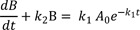
Eq. (5) can be solved simply by noting that

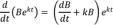
By multiplying both sides of Eq. (5) by e^k₂t and using the above relationship, we get

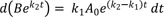
If k₁ ≠ k₂, integration of Eq. (6) from t = 0 to t gives

In the special case when k₁ = k₂, Eq. (6) can reduce to

Then, the integrated expression becomes

The expression for C can be obtained using the mass balance relationship, C = A₀ − A − B,

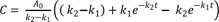
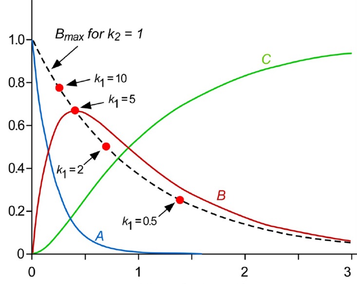
Figure 2 shows a typical amount-time profile of each species for the consecutive first-order irreversible reaction. The amount of A decreases at the normal exponential rate characteristic of a first-order decay curve (blue line). The amount of B follows a bi-exponential profile, first rising and then declining (red line). The amount of C continuously increases and reaches a plateau (green line). This profile is useful for quantifying absorption and elimination processes of drug as well as formation and elimination processes of metabolite.[1314]

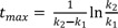
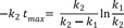
To calculate the maximum amount of B (B_max) and the time to reach the peak (t_max), we take the derivative of Eq. (7), set the derivative, dB/dt, to zero, and rearrange to obtain

Take the natural logarithm of both sides and solve for t_max to get

The resulting B_max at t_max then becomes

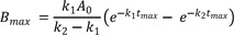
Using Eq. (10), we obtain

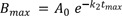
From Eq. (11), we get

Therefore,

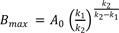
In Figure 2, we also visualized the Equations (11), (13), and (14) to show that t_max decreases and B_max increases as the ratio of k₁ to k₂ increases (dashed line). In other words, when k₂ is smaller than k₁, the amount of A quickly decreases while the amount of B increases rapidly, reaches a maximum at a shorter time, and then falls off with time.

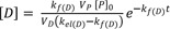
Now consider a case for the intravenous administration of prodrugs (P) in which all the prodrugs are converted to active drugs (D) and then eliminated. In this case, the first-order formation rate constant for D, k_f(D), is equal to the elimination rate constant for P, k_el(P). The parameter k_el(D) represents the first order elimination rate constant for D. The rate of change of D in the blood is determined by the difference between the formation and the elimination rates. Because the level of each species in the blood is measured in concentration ([D] = D/V_D, where V_D is the volume of distribution for D), it is convenient to express Eq. (7) with the same unit. Then, using new notations (k₁ → k_f(D); k₂ → k_el(D)), we get

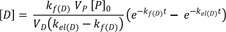
where V_P is the volume of distribution for P, and [P]₀ is the initial concentration of P in the blood.

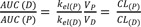
When plasma concentrations are measured as a function of time, the area under the concentration-time curve (AUC) is of great interest in pharmacokinetics. We can derive a useful relationship between AUC and clearance (CL = k×V; volume/time in unit) by solving Eq. (2) using a concentration-time integral method. Writing Eq. (2) in new notations and taking the integral of both sides, we get

Because D is not present in the body initially or at infinity, the left side becomes zero. Rearranging Eq. (16) and substituting k_el(P) = CL_(P)/V_P and k_el(D) = CL_(D)/V_D, we get

This ratio is useful to study metabolic pathway and pharmacokinetic interactions.[891013]

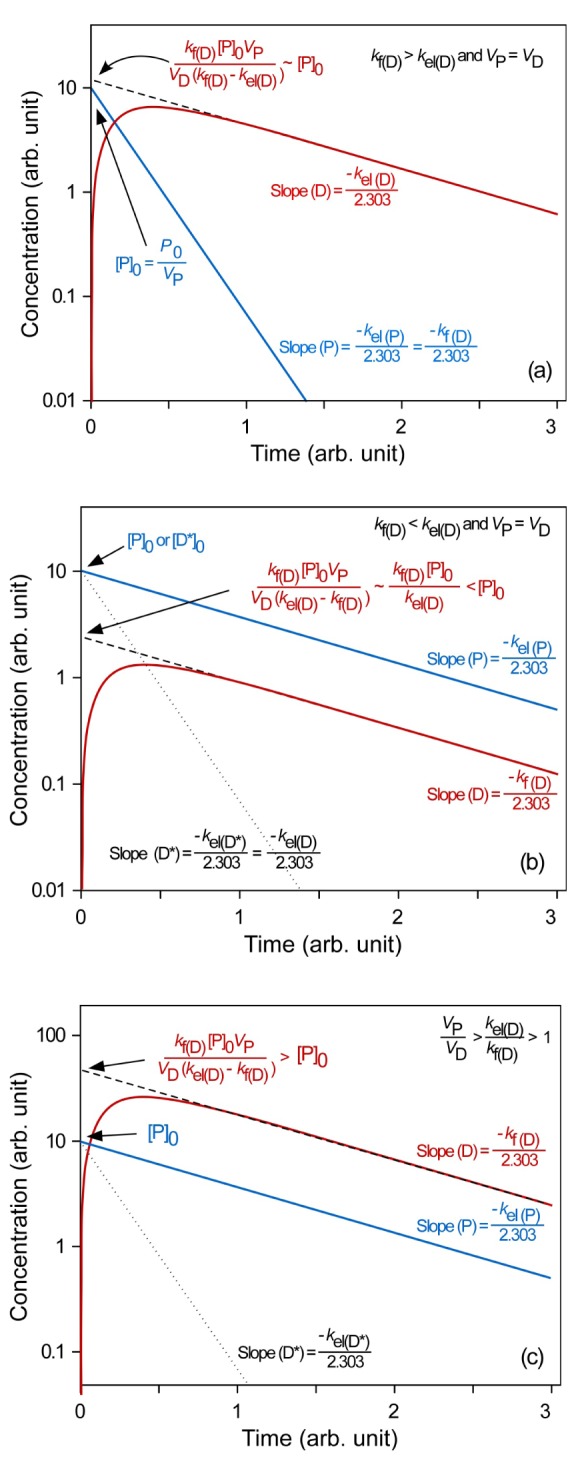
As shown in Eq. (15), the plasma drug concentration, [D], at any given time is expressed by two exponential functions. Depending on the relationship between the prodrug and drug elimination rates, one term can become more dominant than the other. For a more detailed discussion, we consider two limiting situations. In the first situation, formation is a much faster process than elimination (ERL metabolism: k_f(D) > k_el(D)). In the second situation, formation proceeds much more slowly than elimination (FRL metabolism: k_f(D) < k_el(D)). To help understand the underlying kinetics, we simulated these situations to draw semi-logarithmic plots of plasma concentration versus time using Eq. (15) (Fig. 3).

In ERL metabolism, at large time, the first term approaches zero because k_f(D) > k_el(D), and Eq. (15) reduces to

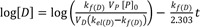
Taking the logarithm to the base 10 of Eq. (18), we get

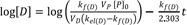
Thus, the semi-logarithmic plots of plasma concentration versus time become linear with a slope of $\frac{k_{el\left(D\right)}}{2.303}$ at large time. Back extrapolation (dashed line) of the elimination phase slope (red line) provides an estimate of [D]₀, which is the intercept of $\frac{k_{f\left(D\right)}{V}_P{\left[P\right]}_0}{V_D\left(k_{f\left(D\right)}-k_{el\left(D\right)}\right)}$ (Fig. 3a). When k_f(D) >> k_el(D) and V_P = V_D, the intercept can be further reduced to [P]₀.

This situation is commonly encountered in the metabolism of many prodrugs.[1015] An example is the metabolism of an antitrypanosomal compound (OSU-36) after an intravenous administration of its ester prodrug (OSU-40) to rat. The hydrolysis of OSU-40 was fast, and its concentrations declined rapidly with short half-life (4.8 min). Whereas, the concentrations of OSU-36, hydrolyzed from OSU-40, declined slowly with the half-life of 41.9 min. This was close to the elimination half-life of the preformed OSU-36 (43.9 min), directly administered to the systemic circulation by an intravenous injection.[15]

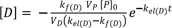
In FRL metabolism (k_f(D) < k_el(D)), at large time, Eq. (15) can be reduced in a similar way to give

and

The slope and intercept of the semi-logarithmic plot of plasma concentration versus time are $\frac{k_{f\left(D\right)}}{2.303}$ and $\frac{k_{f\left(D\right)}{V}_P{\left[P\right]}_0}{V_D\left(k_{el\left(D\right)}-k_{f\left(D\right)}\right)}$, respectively (Fig. 3b). In the elimination phase, thus, the concentration of the parent drug is governed by the prodrug formation rate, not by the prodrug elimination rate. Since k_f(D) < k_el(D), the intercept can be further reduced to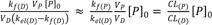

The plasma prodrug concentration, [P], at any given time is easily obtained from Eq. (4), and its final semi-logarithmic expression is

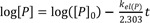
In equations (21) and (23), it is worthwhile to note that the slopes are the same, that is, the concentrations of the parent drug and prodrug decline in parallel (Fig. 3b). Because the parent drug is eliminated almost as soon as it is formed, the elimination rate is approximately equal to the formation rate. The above equation can also be used to plot the plasma concentration-time profile of a preformed D (D*) directly administered to the systemic circulation by an intravenous injection (dotted line). From Figure 3b, we can easily figure out that the half-life of the formed parent drug (ln 2/k_f(D)) in the elimination phase is longer than that of the preformed parent drug (ln 2/k_el(D*)). The half-life of the formed parent drug reflects that of the prodrug (ln 2/k_el(P) = ln 2/k_f(D)).

The FRL metabolism is less encountered in prodrug kinetics but occasionally in metabolite kinetics.[101316] One interesting example is the metabolism of 3′-azido-2′,3′-dideoxy-5′-O-oxalatoylthymidine (AZT-Ac) to zidovudine, [3′-azido-2′,3′-dideoxythymidine (AZT)].[16] Only AZT was detected in plasma, indicating that the prodrug is rapidly hydrolyzed in vivo with a high elimination rate constant. Thus, the first step looks like proceeding according to ERL-metabolism. However, the concentrations of AZT metabolized from AZT-Ac (t_1/2 = 2.16 h) declined more slowly than those of AZT from preformed AZT (t_1/2 = 0.96 h). This means that the metabolic pathway proceeds according to FRL metabolism (k_f(AZT) < k_el(AZT)), as discussed above. This discrepancy may be explained by the presence of multiple pathways for AZT-Ac elimination (small f in Fig. 1) or by the presence of another intermediate between AZT-Ac and AZT. Because AUC for AZT metabolized from AZT-Ac is slightly larger than that for AZT from preformed AZT at the same intravenous dose, the latter explanation looks more plausible.

In FRL metabolism, it is interesting to consider one more situation where V_P/V_D > k_el(D)/k_f(D) > 1, or CL_(P) > CL_(D). As shown in Figure 3c, the intercept for the parent drug ([D]₀) is greater than that for the prodrug ([P]₀). This situation is encountered in the metabolic conversion of propranolol to naphthoxylactic acid (NLA) after single intravenous and oral doses.[17] The AUC of NLA was two times greater than that of propranolol after an intravenous dose of propranolol (4 mg) and ten times after a single oral dose (20 or 80 mg). This can be easily explained if the volume of distribution of NLA is much smaller than that of propranolol. The volumes of distribution of basic drugs are often larger than 100 L, while those of their acidic metabolites are close to 10~20 L.[13] Thus, this situation is expected to be common when a basic prodrug is converted to an acidic parent drug.

We described the prodrug kinetics for the simplest situation: formation and sequential elimination. We can consider a more complicated model to account for more realistic situations but will lose simplicity by including more terms in equations. A more detailed discussion is beyond the scope of this tutorial. For further study, we recommend to read articles and book chapters in the References section.