

 PDF
PDF ePub
ePub Citation
 Print
Print


Introduction
One of most important steps in pharmacometric (PM) analysis is simulation of various scenarios. Among the many software packages used in PM analysis, NONMEM[1] is still accepted as the gold standard, although the user interface is not as good as other software and it has a steep learning curve.
The purpose of this tutorial is to compare the characteristics of NONMEM, Berkeley Madonna,[2] and R[3] by simulating PM models. It is very important for the modeler to have various software options because the appropriate method can vary depending on who will see the PM analysis results. In this tutorial, we will not introduce the detailed analysis procedure for each program, as our intended audience is those who have a basic understanding of modeling using NONMEM. There are also some excellent tutorials available for PM model simulation using Berkeley Madonna[4] and R.[56] The main focus of this manuscript is learning the components of simulation code and the model translation method of this software by working with simple models such as the 2-compartment pharmacokinetic (PK) model and turnover pharmacodynamic (PD) model, as well as dosage regimen adjustment and incorporation of interindividual variability. More complex structural models such as the physiologically-based PK model, target-mediated drug disposition model, complex absorption models, and categorical data simulations will be covered in the next tutorial.
Software
In this tutorial, we will use NONMEM 7.3, Berkeley Madonna 8.3.18, R 3.3.2, and RStudio 1.0.136.[7] NONMEM was developed by ICON Development Solutions (http://www.iconplc.com/technology/products/nonmem/) under a proprietary software license. Berkeley Madonna also requires a license purchase, but most models can be run with the demo version except functions such as ‘save model file’ and ‘export model result.’ R was released under an open-source license.
Example
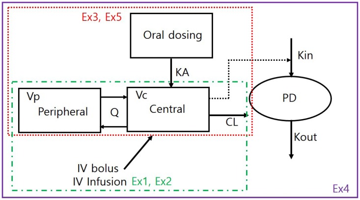
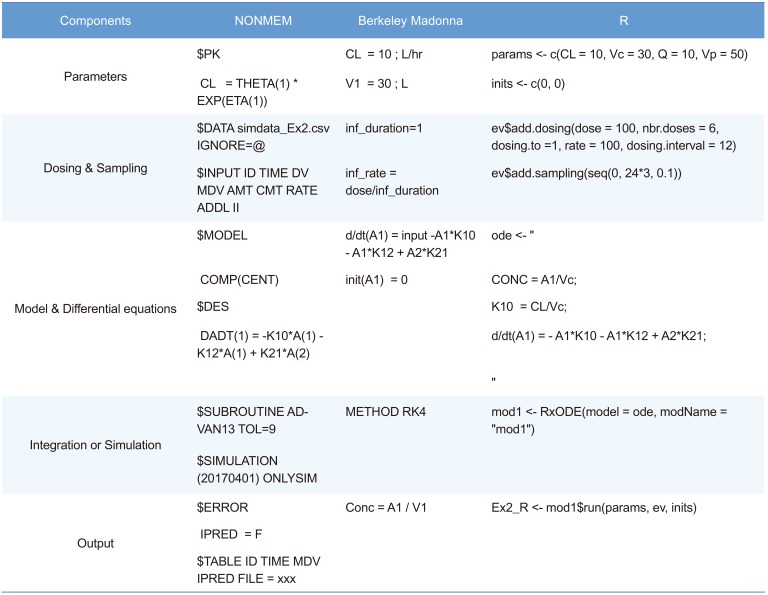
A simple PK/PD model is used to examine structural model change, dosage regimen adjustment, and incorporation of population variability. The structural model used in the simulation is a 2-compartment disposition PK, inhibition of Kin (synthesis rate of PD) turnover PD model (Fig. 1). Table 1 compares software-specific examples of the simulation code components such as parameters, dosing, sampling, differential equation, integration, and output of the simulation.
Example 1: 2-compartment intravenous (IV) bolus PK
NONMEM
In the first example, we assumed a 2-compartment IV bolus PK model result. The parameters were clearance (CL), central volume (Vc), inter-compartmental CL (Q), and peripheral volume (Vp), which were 10 L/hr, 30 L, 10 L/hr, and 50 L, respectively. For the convenience of explanation, there was no inter-individual variability (all OMEGA values were fixed to 0) and residual variability was minimal (additive and proportional error were 0.001 and 0.01). However, because the individual prediction (IPRED), a simulation result of inter-individual variability in the structural model, was used for comparison of the simulation results, residual variability had no effect on simulation performance. In terms of how to perform the simulation, the biggest difference between NONMEM and other software is the necessity of a simulation dataset for simulation in NONMEM. Dosage regimens or sampling points were set in the simulation dataset. The NONMEM code is presented in the following section. Although a 2-compartment IV bolus model can be implemented using ADVAN3 in NONMEM, ADVAN13 (or ADVAN 6) was used because comparison of differential equation models was the main purpose of this tutorial. $MODEL defines the compartments of the model, and PK parameters are defined using the THETA (n) and ETA(n) in $PK. In $DES, differential equations are constructed with appropriate rules. In $ERROR, the gap between individual prediction (IPRED) and observation can be set with residual error. Finally, the variables needed for comparison of the simulation results were stored in a table file for post-processing with R.
$PROB Ex1_2-compartment IV bolus
$DATA simdata_Ex1.csv IGNORE=@
$INPUT ID TIME DV MDV AMT CMT
$SUBROUTINE ADVAN13 TOL=9
$MODEL
$PK
$DES
DADT(1) = -K10*A(1) - K12*A(1) +K21*A(2)
DADT(2) = K12*A(1) - K21*A(2)
$ERROR
$THETA
$OMEGA
$SIGMA
$SIMULATION (20170401) ONLYSIM
$TABLE ID TIME AMT DV MDV IPRED PRED ONEHEADER NOPRINT NOAPPEND
FILE = Ex1_NM
Berkeley Madonna
METHOD, STARTTIME and STOPTIME specify the integration method (RK4; Runge–Kutta 4), start time and stop time of the integration interval. The default integration method is RK4, but other methods such as Euler, RK2, Auto, and Stiff are also available; please refer to the ‘ODE SOLVERS’ section of the reference.[4] DT and DTOUT define the time intervals to be used in the numerical solution of the differential equation system and output time interval, respectively. The default value of DTOUT is zero, and if set to zero, the time interval of DT is applied to the simulation output. Note that the smaller the DT, the longer the time required for the simulation. However, if the DT is too large, the simulation result may change. Therefore, it is necessary to check the difference in simulation results according to the DT. The PK parameter setting is the same as in NONMEM, but direct values are used instead of terms such as THETA and ETA. The differential equations are nearly the same. There are several syntax options for defining differential equations, but the following two methods are the most commonly used.
In NONMEM, since the default value of the compartment at time 0 is 0, the syntax error does not occur even if the compartment value is not specified; however, in Berkeley Madonna, an initial compartment value must be specified even if it is 0. In the case of IV bolus, the initial dose of the central compartment was set as the dose administered. In NONMEM, the scale parameter is reflected and the simulated data represent concentration instead of the amount. However, the Berkeley Madonna does not have such a function, so users must directly define the concentration using the amount and appropriate parameters such as the volume of distribution of central compartment. A ‘DISPLAY’ statement is not mandatory, but you can control which variables are included in the built-in plot window. To specify the variable name to be included in the slider, write DISPLAY again. The sliders window provides a convenient way of changing parameters and automatically running the model. It is common practice to export the data table as a text or comma-separated value (csv) file. In the Berkeley Madonna graph window, clicking on the icon displays two squares partially overlaid. The resulting table gives the data shown in the visual display. The menu “File Save Table As” now allows storage of data as a text or csv file.
R
To solve the differential equation using R, a differential equation solver is required. The default solver provided in R is the ‘deSolve’ package. However, pharmacometric model simulation using the ‘deSolve’ package requires much more complex R coding for dosing regimens or sampling design. Several packages such as ‘PKPDsim,’ ‘RxODE,’ and ‘mrgsolve’ have been developed to overcome these drawbacks. In this tutorial, we used the ‘RxODE’ package because of the ease of comparison with other codes and the author's experience of using this package for simulation in R. A detailed description of ‘RxODE’ and R codes with various examples are provided in the supplementary material in the reference [6]. To use the ‘RxODE’ package, you need to install it by running the following script in the console. Windows users will need to have the appropriate version of Rtools installed. ‘RxODE’ is available on Github at (https://github.com/hallowkm/RxODE) and detailed instructions are provided on this site.
The code structure and the writing of differential equations are very similar to those of the Berkeley Madonna. A compilation manager translates the ODE model into C, compiles it, and dynamically loads the object code into R for improved computational efficiency.[8] Each equation is separated by a semicolon. Dosing and sampling design can be set very intuitively using ‘eventTable.’ An event table object facilitates the specification of complex dosing regimens and sampling schedules. Detailed examples and methods are described in the reference.[6]
Example 2: 2-compartment IV infusion PK and adjustment for dosage regimen
NONMEM
IV infusion can be controlled by the infusion rate and duration. To control the infusion rate in NONMEM, users need to enter the amount to be infused per unit time into the RATE column of the dataset. In Example 2, infusion time is automatically defined as the amount / rate (100 mg / 100 mg/hr = 1 hr). Repeated dosing and dosing intervals should be adjusted in the simulation dataset. The dosage regimen can be controlled using ADDL and II columns. In Example 2, we will show an example of dosing every 12 hr for 3 days. To set up this dosage regimen, set ADDL as 5 and II as 12, and sampling time points should be 0–72 hr. There is no change in the control file except that ADDL and II columns are added to $ INPUT.
Berkeley Madonna
In addition to implementing IV infusion, we will look at codes that allow flexible setting of the number of doses and dosing interval in Berkeley Madonna. First, dose, duration of infusion, infusion rate, dosing interval, and number of doses are set to dose, inf_duration, inf_rate, inf_interval, and ndoses. The ‘is_inftime’ variable is an indicator that allocates 1 during the infusion and 0 for after the infusion ends. The ‘dosingperiod’ is also an indicator variable determined by the number of doses (ndoses) and dosing interval (inf_interval): 1 for the period where dosing is going on and 0 for the period without dosing. The actual infusion consists of a combination of three variables, inf_rate, is_inftime, and dosingperiod, which are assigned to the ‘input’ variable. The input is incorporated in the dosing compartment of the differential equation (in this case, A1).
…
{Differential equations}
d/dt(A1) = input - A1*K10 –A1*K12 + A2*K21
d/dt(A2) = A1*K12 - A2*K21
…
{Dosing}
dose = 100 ; dose administered (mg)
inf_duration=1 ;infusion duration (h)
inf_rate = dose/inf_duration ; infusion rate (units/h)
inf_interval=12 ; infusion interval for multiple dosing (h)
ndoses=6
is_inftime=(time >= 0) and (mod(time, inf_interval) < inf_duration)
dosingperiod = if time < ndoses * inf_interval then 1 else 0
input = inf_rate * is_inftime * dosingperiod
Example 3: 2-compartment, first-order absorption Oral PK
NONMEM
Implementation of oral absorption is relatively simple. An absorption compartment should be added to $MODEL, a differential equation for first-order absorption in $DES, and a first-order absorption rate constant (KA) parameter are also added to $PK.
$MODEL
COMP(DEPOT)
COMP(CENT)
COMP(PERIPH)
$PK
…
KA = THETA(5) * EXP(ETA(5))
…
$DES
DADT(1) = -KA*A(1)
DADT(2) = KA*A(1) - K20*A(2) - K23*A(2) + K32*A(3)
DADT(3) = K23*A(2) - K32*A(3)
In this case, dosing is entered in the absorption compartment (CMT=1) and the observation is made in the central compartment (CMT=2), so the number of CMT columns in the simulation dataset must be adjusted accordingly.
Berkeley Madonna
The Berkeley Madonna also requires an additional compartment, differential equation, and KA parameter. Since it is not an infusion, only the indicator of the dosing period is set up for repeated administration. After defining the input variable using the pulse function, we put the input into the A1 compartment. The ‘pulse’ function, which is a Berkeley Madonna built-in function that allows you to set the dose, lag time, and dosing interval, is often used in dosing settings.
;Differential equations
d/dt(A1) = input - KA*A1
d/dt(A2) = KA*A1 - K20*A2 –K23*A2 + K32*A3
d/dt(A3) = K23*A2 - K32*A3
init(A1) = 0
init(A2) = 0
init(A3) = 0
;Dosing input.
;Set to zero after ndoses administered
dosingperiod = if time < ndoses * dose_int then 1 else 0
input = pulse(dose, 0, dose_int) * dosingperiod
Example 4: 2-compartment Oral PK & turnover (Kin inhibition) PD model
NONMEM
First, the sampling points of the observation compartment in the simulation dataset should be set to PK and PD, respectively, and distinguished in the CMT column. Therefore, PD sampling is added to the existing dataset and the compartment number is set to 4. The R code for dataset generation is as follows.
In the control file, it is necessary to set the initial value of the PD compartment as baseline (A_0(4) =
BASE) in addition to adding the PD compartment to the $MODEL defining the PD parameter and correcting the differential equation. Since PK and PD observations must be computed separately, we set the error models for CMTs of 2 and 4 at $ERROR, respectively.
$MODEL
COMP(DEPOT)
COMP(CENT)
COMP(PERIPH)
COMP(EFFECT)
$PK
…
;PD
BASE = THETA(6) * EXP(ETA(6))
KOUT = THETA(7) * EXP(ETA(7))
EC50 = THETA(8) * EXP(ETA(8))
EMAX = THETA(9) * EXP(ETA(9))
KIN = BASE * KOUT
A_0(4) = BASE
…
$DES
CONC = A(2)/S2
DADT(1) = -KA*A(1)
DADT(2) = KA*A(1) - K20*A(2) - K23*A(2) + K32*A(3)
DADT(3) = K23*A(2) - K32*A(3)
EFF = EMAX*CONC / (EC50 + CONC)
DADT(4) = KIN*(1-EFF) - KOUT*A(4)
$ERROR
IF (CMT.EQ.2) THEN
IPRED = A(2)/S2
W = SQRT(THETA(10)**2 + THETA(11)**2 * IPRED**2)
ENDIF
IF (CMT.EQ.4) THEN
IPRED = A(4)
W = SQRT(THETA(12)**2)
ENDIF
IRES = DV - IPRED
IWRES = IRES / W
Y = IPRED + W * EPS(1)
Berkeley Madonna
PD compartment, differential equation, PD parameters, and initial value of the PD compartment are set. The changes compared to Example 3 are as follows.
{PD parameters}
BASE = 100
KOUT = 0.5
EC50 = 0.5
EMAX = 1
KIN = BASE * KOUT
{Differential equations}
Conc = A2 / V2
d/dt(A1) = input - KA*A1
d/dt(A2) = KA*A1 - K20*A2 - K23*A2 + K32*A3
d/dt(A3) = K23*A2 - K32*A3
EFF = EMAX*Conc / (EC50 + Conc)
d/dt(A4) = KIN*(1-EFF) - KOUT*A4
init(A1) = 0
init(A2) = 0
init(A3) = 0
init(A4) = BASE
R
The same principle applies to R, and the part of the code that is changed is as follows.
ode 〈- "
CONC = A2/Vc;
K12 = KA;
K20 = CL/Vc;
K23 = Q/Vc;
K32 = Q/Vp;
d/dt(A1) = -A1*K12;
d/dt(A2) = A1*K12 - A2*K20 - A2*K23 + A3*K32;
d/dt(A3) = A2*K23 - A3*K32;
KIN = BASE*KOUT;
EFF = EMAX*CONC / (EC50+CONC);
PD = A4;
d/dt(A4) = KIN*(1-EFF) - A4*KOUT;
"
# Compile model
mod1 〈- RxODE(model = ode,
modName = “mod1”)
# Define system parameters
Base = 100
Kout = 0.5
params 〈- c(KA = 1,CL = 10,Vc = 30,
Q = 10, Vp = 50,
EMAX = 1,EC50 = 0.5,
BASE = Base,KOUT = Kout)
inits 〈- c(0, 0, 0, Base)
Example 5: Population simulation
NONMEM
Example 5 simulates 1000 individuals with 20% variability in CL, Vc, and Ka with the 2-compartment oral PK model. The only changes are the number of ID (nID) value from 1 to 1000 in the dataset simulation code, and $OMEGA in the NONMEM control file given as 0.04 for CL, Vc, and Ka instead of ‘0 FIX.’
Berkeley Madonna
In Berkeley Madonna, array equations are useful tools that can be used for many purposes. One-dimensional arrays (vectors) are defined as follows:
Arrays of differential equations are defined by placing the brackets immediately following the variable name. For example, the following equations define a set of N differential equations:
In addition to the number of ID (N) and standard deviation of the parameter (CLsd, V2sd, KAsd), most of the code has been changed to the array type compared with the Ex3 code.
{Ex5 2-compartment Oral, population simulation}
METHOD RK4 ; Integration method
STARTTIME =0
STOPTIME = 24
DT = 0.001 ; Integration time step
DTOUT = 0.1 ; Output time interval
N = 1000
{Population PK parameters}
CLpop = 10 ; L/hr
V2pop = 30 ; L
Q = 10 ; L/hr
V3 = 50 ; L
KApop = 1 ; 1/hr
{Standard deviation of PK parameters}
CLsd = 0.2
V2sd = 0.2
KAsd = 0.2
{Generate random effetcs on CL,V2,KA}
init eta_CL[1..N] = NORMAL(0,1)*CLsd
init eta_V2[1..N] = NORMAL(0,1)*V2sd
init eta_KA[1..N] = NORMAL(0,1)*KAsd
next eta_CL[1..N] = eta_CL[i]
next eta_V2[1..N] = eta_V2[i]
next eta_KA[1..N] = eta_KA[i]
CL[1..N] = CLpop * exp(eta_CL[i])
V2[1..N] = V2pop * exp(eta_V2[i])
KA[1..N] = KApop * exp(eta_KA[i])
K20[1..N] = CL[i]/V2[i]
K23[1..N] = Q/V2[i]
K32[1..N] = Q/V3
{Differential equations}
d/dt(A1[1..N]) = input[i]
- KA[i]*A1[i]
d/dt(A2[1..N]) = KA[i]*A1[i]
- K20[i]*A2[i]
- K23[i]*A2[i]
+ K32[i]*A3[i]
d/dt(A3[1..N]) = K23[i]*A2[i]
- K32[i]*A3[i]
init A1[1..N] = 0
init A2[1..N] = 0
init A3[1..N] = 0
{Dosing}
dose = 100 ; mg
dose_int=24 ; dosing interval
ndoses=1 ; number of doses
idose[1..N] = dose
idose_int[1..N] = dose_int
indoses[1..N] = ndoses
dosingperiod[1..N] = if time < indoses[i]*idose_int[i] then 1 else 0
input[1..N] = pulse(idose[i],0, idose_int[i]) *dosingperiod[i]
{Output}
Conc[1..N] = A2[i] / V2[i]
DISPLAY Conc
DISPLAY CLpop,V2pop,Q,V3,KApop,CLsd, V2sd,KAsd,dose,ndoses,dose_int,N
R
In R, we need to generate an individual ETA matrix to reflect interindividual variability. In this tutorial, the ‘mvrnorm’ function of the ‘MASS’ package was utilized and an individual parameter matrix was generated. Each individual was simulated by looping through the parameter matrix, using each row as an input for the simulation, and collecting the output of each simulation in an output matrix.
library(RxODE)
library(ggplot2)
library(MASS)
nsub 〈- 1000
sigma 〈- matrix(c(0.04, 0, 0,
0, 0.04, 0,
0, 0,0.04),
3, 3)
mv 〈- mvrnorm(n = nsub,
rep(0,3), sigma)
# Define model
ode 〈- "
CONC = A2/Vc;
K20 = CL/Vc;
K23 = Q/Vc;
K32 = Q/Vp;
d/dt(A1) = -A1*KA;
d/dt(A2) = A1*KA - A2*K20
– A2*K23 + A3*K32;
d/dt(A3) = A2*K23 - A3*K32;
"
# Compile model
mod1 〈- RxODE(model = ode,
modName = “mod1”)
# Define system parameters
CLpop = 10
Vcpop = 30
KApop = 1
CL = CLpop*exp(mv[,1])
Vc = Vcpop*exp(mv[,2])
KA = KApop*exp(mv[,3])
params.all 〈-
cbind(KA=KA, CL=CL,
Vc=Vc, Q=10, Vp=50)
inits 〈- c(0, 0, 0)
# Initialize event table
ev 〈- eventTable()
ev$add.dosing(dose = 100,
nbr.doses = 1,
dosing.to =1)
ev$add.sampling(seq(0, 24, 0.1))
Ex5 〈- NULL
for (i in 1:nsub) {
params 〈- params.all[i,]
x 〈- mod1$run(params,
ev,
inits = inits)
Ex5 〈- cbind(Ex5,x[,“CONC”])
}
Summary
We compared the PM simulation method using three different programs. Simulation with NONMEM is relatively convenient because it can be used almost without modifying original code if only simulation dataset is created, but NONMEM is not suitable for interactive simulations such as changes in the PK / PD profile according to parameter changes. BM is very useful for sensitivity analysis using slides, while complicated dosing regimens or population simulations require complex code modifications. R is somewhat complicated to simulate with its own functions, but since useful packages are being developed, there is a difference in the degree of convenience depending on how R is used. Although it is not introduced in this tutorial, R is a good option for PM modelers because many interactive applications using R Shiny have been developed.[59]
 XML Download