Journal List > Transl Clin Pharmacol > v.25(2) > 1142669

Bae and Kang: Bioequivalence data analysis for the case of separate hospitalization

Abstract

A bioequivalence study is usually conducted with the same-day drug administration. However, hospitalization is occasionally separated for logistical, operational, or other reasons. Recently, there was a case of separate hospitalization because of difficulties in subject recruitment. This article suggests a better way of bioequivalence data analysis for the case of separate hospitalization. The key features are (1) considering the hospitalization date as a random effect than a fixed effect and 2) using “PROC MIXED” instead of “PROC GLM” to include incomplete subject data.

Introduction

Determining a final model among many competitive models is usually not a matter of “right or wrong” but of “better or worse.” In other words, it is important to remember the famous statement by George Box, “All models are wrong, but some are useful.”
A result of bioequivalence study with separate hospitalization was discussed at the Central Pharmaceutical Affairs Advisory Committee (CPAC) by the Korea Ministry of Food and Drug Safety (MFDS) in January 2017. The content of this article is the authors' opinion as expert advisors. The sponsor company agreed on the publication this information and provided the data for this article.
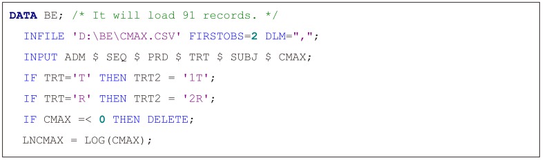
Methods

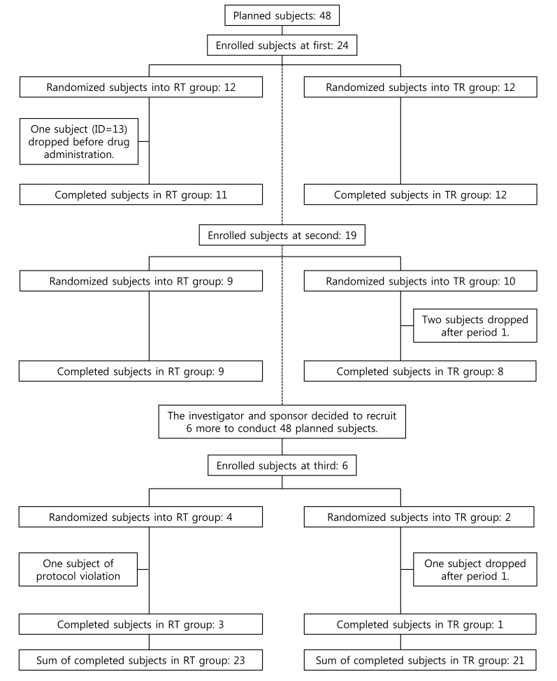
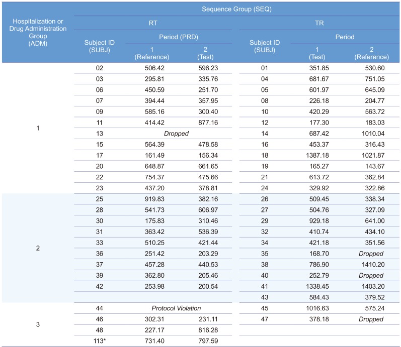
A 2×2 bioequivalence study was planned to include 24 subjects for each of the two treatment sequence groups (48 subjects in total). The study requested the subjects to have long period of hospitalization with strict inhibition of sunlight exposure. Therefore, there were not many volunteers for this condition. Subject disposition is shown in Figure 1 and maximum concentration (Cmax) data is listed in Table 1.
SAS® 9.4 was used for data analysis; the script for data loading and an explanation of variable names are specified in Figure 2. At least 10 data analysis models, from the most naïve to the most complex ones, were considered (Table 2).

Results

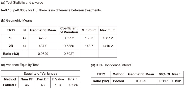
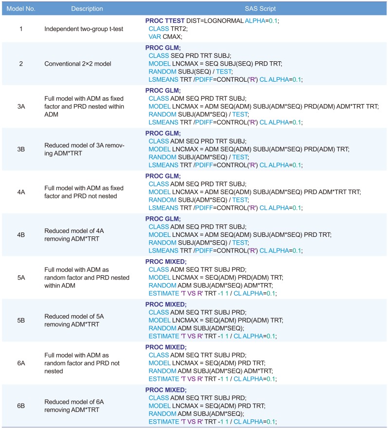
Model 1. Independent two-group t-test

Figure 3 shows the summary of results of the independent two-group t-test, the most naïve approach. The equality of variances between the treatments could be assumed (p=0.8986), and the null hypothesis (i.e., there is no difference between the treatments) could not be rejected (p=0.8809). The width of 90% confidence interval (CI) for the geometric mean ratio was 0.3784, which is relatively wide and means the most inefficient method presented in Table 2. However, the bioequivalence of the test treatment, within the limit of [0.8, 1.25], was observed. However, this model is not acceptable as a final model by any regulatory body. Current regulatory guidelines request bioequivalence study to include the effects such as sequence, period, and random subject effect nested within the sequence in the final model.

Model 2. Conventional 2×2 model

If we ignore the effect of separate hospitalization (drug administration), the final model could be the conventional 2×2 crossover bioequivalence study model (Fig. 4). This model can only be used after the full model (considering the effect of separate hospitalization) is examined and when the additional effects such as hospitalization date can be ignored. This was the final model of the sponsor company after consulting a professor of statistics who advised that those insignificant additional effects (hospitalization and its interaction effects) could be removed.

Model 3A. Full model with administration (ADM) as fixed factor and period (PRD) nested within ADM

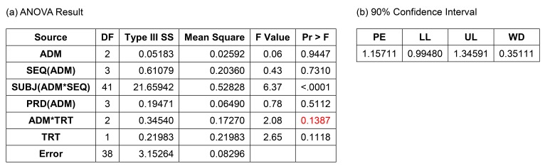
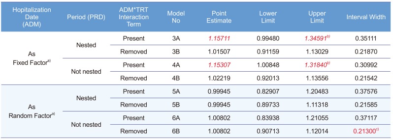
Figure 5 shows the result of this model. The interaction term between ADM and treatment was not significant (p = 0.1387), and many statisticians would agree to remove this term. The 90% CI (0.99480–1.34591) did not meet the bioequivalence limit, which was the main reason why the Korea MFDS summoned CPAC. In fact, European Medicines Agency (EMA) prohibited this kind of analysis, but some CPAC members wanted this to be the final model or analysis.

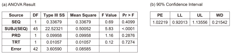
Model 3B. Reduced model of 3A by removing the interaction term between ADM and treatment

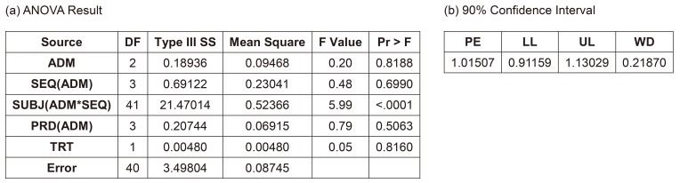
After removing the insignificant interaction term, the CI (0.91159–1.13029) satisfied the bioequivalence criteria, and the analysis of variance (ANOVA) result was acceptable (Fig. 6). Many statisticians would be comfortable with this as a final model. A more simplified model, such as Model 2, would also be acceptable. The ANOVA table shows satisfactory F values for further pooling of the terms into the error term to increase the efficiency of the estimation, which are explained in the statistics textbooks of experimental designs.[1] A rule of thumb for pooling is “F ≤1.” This model is the same one that the EMA suggested.[2]

Model 4A. Full model with ADM as fixed factor and PRD not nested

The EMA suggests using Model 3B, in which PRD is nested within the ADM. However, some may consider PRD as not-being nested. The ANOVA result are not much different (data not shown), the CIs of this and other models are summarized in Table 3. This model along with all the following models showed desirable ANOVA results and satisfied the bioequivalence criteria.

Model 4B. Reduced model of 4A by removing the interaction term between ADM and treatment

After removing the insignificant interaction term, the result met the bioequivalence criteria. The confidence limit is summarized in Table 3.

Model 5A–6B. Models considering ADM as a random factor and using PROC MIXED to include the subject data with PRD 1 only

The Models 5A–6B corresponded to Models 3A–4B, respectively, using PROC MIXED instead of PROC GLM for the CI calculation. PROC MIXED used the data of subjects who dropped out after PRD 1, whereas PROC GLM did not. Another important difference of these models is considering ADM as a random factor based on the statistics textbook.[1] Models 5A and 5B seem controversial because some consider that a fixed factor (PRD) nested within a random factor (ADM) should be a random factor.[3] All models examined here showed satisfactory results and met the equivalence criteria. The CIs are summarized in Table 3. Model 6B was the most efficient model and showed the narrowest CI (Table 3). In addition, Models 3A and 4A show seemingly biased point estimations compared with the other models.

Discussion

All acquired data during the trial should be included, if they increase the precision, and do not cause more bias. Thus, we suggest that using PROC MIXED is better than using PROC GLM. Many references comparing PROC MIXED and PROC GLM are available recently.[456]
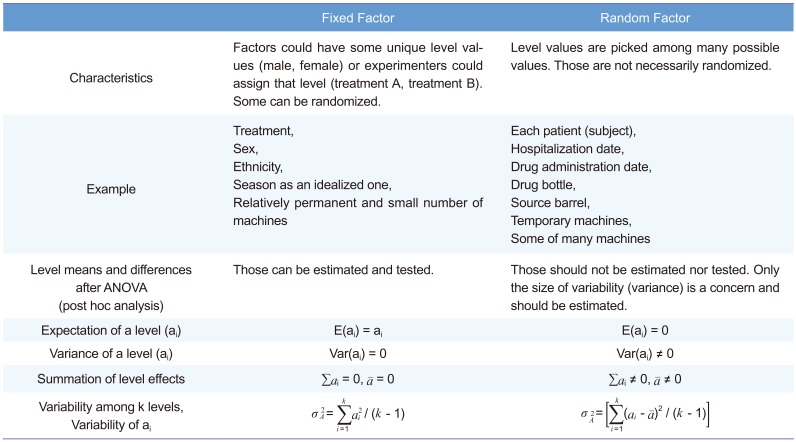
Another point of discussion is how to deal with the drug ADM (hospitalization) date as a fixed or a random effect. We strongly suggest that this effect should be considered random, following the textbook[1] written by Sung Hyun Park, a professor of statistics at Seoul National University and president of the South Korean Academy of Science and Technology. Many other references also support that.[3,7891011] Table 4 summarizes the fixed versus random factor concept. For both fixed and random factors, randomization is easy for some (treatment for fixed factor, drug bottle for random factor), while difficult for some others (sex for fixed factor, hospitalization date for random factor). Therefore, randomization is not a classification criterion.
Precision or efficiency (small or minimum variance) is one of the criteria used to judge whether an estimation is good or not. If bias is not a problem, a more precise estimation will result in a narrower CI. As seen in Table 3, Model 6B was the most efficient (CI width, 0.21300), and Model 6B is likely to be less biased than Models 3A or 4A. A possible reason for Models 3A and 4A being biased and less efficient can be found in the following paragraph from the EMA[2]:
A model which also includes a term for a formulation*stage interaction would give equal weight to the two stages, even if the number of subjects in each stage is very different. The results can be very misleading; hence, such a model is not considered acceptable. Furthermore, this model assumes that the formulation effect is truly different in each stage. If such an assumption were true, there is no single formulation effect that can be applied to the general population, and the estimate from the study has no real meaning.
Conclusion
...
3) A term for a formulation*stage interaction should not be fitted.
“Formulation” and “stage” in the above passage are equivalent to “treatment” and “hospitalization,” respectively, in the present article.
Many more models can be considered with different arrangement of effect terms. However, all important models are addressed here.
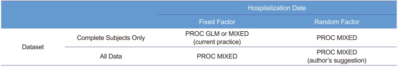
In a retrospective view, the third hospitalization should not be done, because the sample size of the earlier two hospitalization groups appeared sufficient (post hoc power analysis indicated 16 subjects/group achieved a power of 80%[12]), whereas the third hospitalization group was too small to be balanced. With one subject drop, the allocation ratio became 3:1. Therefore, one seemingly outlier subject (ID: 48) had high influence on the third group, which in turn had too much weight for the estimation, if we had used a fixed effect model. Meanwhile, random effect models of ADM were resistant to this kind of bias or outlier. In practice, we could not assign or specify ADM at the time of protocol development or trial planning nor could we reproduce that date effect thereafter. Moreover, ADM could not (and should not) be the concern of the fixed effect (i.e., the level means of specific dates are not our concern). A very large inter-day variability compared with that of the treatment effect can be a concern for doctors. However, this was not the case (F <1). Therefore, the authors insist the use of a random effect model for the hospitalization (or drug administration) date to increase efficiency and robustness. Table 5 shows the comparison of PROC MIXED and PROC GLM to help choosing a procedure.
Our prescriptive conclusions are summarized below from the highest to lowest priority:
  1. Treat hospitalization date as a random factor

  2. Use PROC MIXED rather than PROC GLM to use all acquired data

  3. Do not nest period within hospitalization date

Acknowledgements

The authors would like to thank Dr. Sungpil Han for helping in proofreading and drawing figures.
This manuscript was to be written as a tutorial or opinion paper when initially invited by the EIC of TCP. However, it was finally written in the format of original article by the opinion of authors.

Notes

Conflict of Interest: The authors declare that they have no conflict of interest.

References

1. Park SH. Design of Experiments. 2nd ed. Seoul: Min-Young Sa;2003. p. 58–60. p. 107–109. p. 146–148.
2. EMA. Questions & Answers: positions on specific questions addressed to the Pharmacokinetics Working Party (PKWP). 2015. p. 32.
Smith MK. Inappropriately Designating a Factor as Fixed or Random. Accessed 1 May 2017. https://www.ma.utexas.edu/users/mks/statmistakes/fixedvsrandom.html.
4. SAS. SAS/STAT 9.3 User's Guide. SAS Institute;2011. p. 217–218.
5. SAS. SAS/STAT 14.1 User's Guide. SAS Institute;2015. p. 123.
6. Elliott AC, Woodward WA. SAS Essentials: Mastering SAS for Data Analytics. 2nd ed. Wiley;2015.
7. Galwey NW. Introduction to Mixed Modeling: Beyond Regression and Analysis of Variance. 2nd ed. Wiley;2014.
8. Haney SA, Bowman D, Chakravarty A, Davies A, Shamu C. An Introduction to High Content Screening: Imaging Technology, Assay Development, and Data Analysis in Biology and Drug Discovery. Wiley;2015.
9. Torbeck LD. Pharmaceutical and Medical Device Validation by Experimental Design. CRC Press;2017.
10. Aris VM. 8. Using microarrays to measure cellular changes induced by biomaterials. Characterization of biomaterials. Woodhead Publishing;2012.
11. Gibson D. Methods in Comparative Plant Population Ecology. 2nd ed. Oxford University Press;2014.
12. Diletti E, Hauschke D, Steinijans VW. Sample size determination for bioequivalence assessment by means of confidence intervals. Int J Clin Pharmacol Ther Toxicol. 1992; 30(Suppl 1):S51–S58. PMID: 1601532.
Figure 1

Subject disposition.

tcp-25-93-g001
Figure 2

SAS script for data loading. ADM, hospitalization (drug administration) group code (1, 2, or 3); SEQ, treatment sequence group (RT, reference then test treatment; TR, test then reference treatment); PRD, period (1 or 2); TRT, treatment (T, test treatment; R, reference treatment); SUBJ, subject ID; CMAX, maximum concentration (Cmax) value in original scale; LNCMAX, Cmax value in natural log scale.

tcp-25-93-g002
Figure 3

Results of the independent two-group t-test.

tcp-25-93-g003
Figure 4

Result of conventional 2 × 2 model (Model 2). (a) ANOVA result, (b) 90% confidence interval, SEQ, treatment sequence group; SUBJ, subject ID; PRD, period; TRT, treatment; PE, point estimate; LL, lower limit; UL, upper limit; WD, width of confidence interval.

tcp-25-93-g004
Figure 5

Result of full Model (3A) with drug administration (ADM) as a fixed factor and period (PRD) nested within ADM. (a) ANOVA result, (b) 90% confidence interval, ANOVA, analysis of variance; SEQ, treatment sequence group; SUBJ, subject ID; TRT, treatment; PE, point estimate; LL, lower limit; UL, upper limit; WD, width of confidence interval.

tcp-25-93-g005
Figure 6

Result of reduced Model (3B) with drug administration (ADM) as a fixed factor and period (PRD) nested within ADM. (a) ANOVA result, (b) 90% confidence interval, ANOVA, analysis of variance; SEQ, treatment sequence group; SUBJ, subject ID; TRT, treatment; PE, point estimate; LL, lower limit; UL, upper limit; WD, width of confidence interval.

tcp-25-93-g006
Table 1

Maximum concentration (Cmax) data before log transformation

tcp-25-93-i001
Hospitalization or Drug Administration Group (ADM) Sequence Group (SEQ)
RT TR
Subject ID (SUBJ) Period (PRD) Subject ID (SUBJ) Period
1 (Reference) 2 (Test) 1 (Test) 2 (Reference)
1 02 506.42 596.23 01 351.85 530.60
03 295.81 335.76 04 681.67 751.05
06 450.59 251.70 05 601.97 645.09
07 394.44 357.95 08 226.18 204.77
09 585.16 300.40 10 420.29 563.72
11 414.42 877.16 12 177.30 183.03
13 Dropped 14 687.42 1010.04
15 564.39 478.58 16 453.37 316.43
17 161.49 156.34 18 1387.18 1021.87
20 648.87 661.65 19 165.27 143.67
22 754.37 475.66 21 613.72 362.84
23 437.20 378.81 24 329.92 322.86
2 25 919.83 382.16 26 509.45 338.34
28 541.73 606.97 27 504.76 327.09
30 175.83 310.46 29 929.18 641.00
31 363.42 536.39 32 410.74 434.10
33 510.25 421.44 34 421.18 351.56
36 251.42 203.29 35 168.70 Dropped
37 457.28 440.53 38 786.90 1410.20
39 362.80 205.46 40 252.79 Dropped
42 253.98 200.54 41 1338.45 1403.20
43 584.43 379.52
3 44 Protocol Violation 45 1016.63 575.24
46 302.31 231.11 47 378.18 Dropped
48 227.17 816.28
113* 731.40 797.59

*Subject 113 is the replacement of subject 13.

Table 2

Ten models for data in Table 1

tcp-25-93-i002
Model No. Description SAS Script
1 Independent two-group t-test PROC TTEST
 DIST=LOGNORMAL ALPHA=0.1;
 CLASS TRT2;
 VAR CMAX;
2 Conventional 2×2 model PROC GLM;
 CLASS SEQ PRD TRT SUBJ;
 MODEL LNCMAX = SEQ SUBJ(SEQ) PRD TRT;
 RANDOM SUBJ(SEQ) / TEST;
 LSMEANS TRT /PDIFF=CONTROL('R') CL ALPHA=0.1;
3A Full model with ADM as fixed factor and PRD nested within ADM PROC GLM;
 CLASS ADM SEQ PRD TRT SUBJ;
 MODEL LNCMAX = ADM SEQ(ADM) SUBJ(ADM*SEQ) PRD(ADM) ADM*TRT TRT;
 RANDOM SUBJ(ADM*SEQ) / TEST;
 LSMEANS TRT /PDIFF=CONTROL('R') CL ALPHA=0.1;
3B Reduced model of 3A remov- ing ADM*TRT PROC GLM;
 CLASS ADM SEQ PRD TRT SUBJ;
 MODEL LNCMAX = ADM SEQ(ADM) SUBJ(ADM*SEQ) PRD(ADM) TRT;
 RANDOM SUBJ(ADM*SEQ) / TEST;
 LSMEANS TRT /PDIFF=CONTROL('R') CL ALPHA=0.1;
4A Full model with ADM as fixed factor and PRD not nested PROC GLM;
 CLASS ADM SEQ PRD TRT SUBJ;
 MODEL LNCMAX = ADM SEQ(ADM) SUBJ(ADM*SEQ) PRD ADM*TRT TRT;
 RANDOM SUBJ(ADM*SEQ) / TEST;
 LSMEANS TRT /PDIFF=CONTROL('R') CL ALPHA=0.1;
4B Reduced model of 4A removing ADM*TRT PROC GLM;
 CLASS ADM SEQ PRD TRT SUBJ;
 MODEL LNCMAX = ADM SEQ(ADM) SUBJ(ADM*SEQ) PRD TRT;
 RANDOM SUBJ(ADM*SEQ) / TEST;
 LSMEANS TRT /PDIFF=CONTROL('R') CL ALPHA=0.1;
5A Full model with ADM as random factor and PRD nested within ADM PROC MIXED;
 CLASS ADM SEQ TRT SUBJ PRD;
 MODEL LNCMAX = SEQ(ADM) PRD(ADM) TRT;
 RANDOM ADM SUBJ(ADM*SEQ) ADM*TRT;
 ESTIMATE 'T VS R' TRT -1 1 / CL ALPHA=0.1;
5B Reduced model of 5A removing ADM*TRT PROC MIXED;
 CLASS ADM SEQ TRT SUBJ PRD;
 MODEL LNCMAX = SEQ(ADM) PRD(ADM) TRT;
 RANDOM ADM SUBJ(ADM*SEQ);
 ESTIMATE 'T VS R' TRT -1 1 / CL ALPHA=0.1;
6A Full model with ADM as random factor and PRD not nested PROC MIXED;
 CLASS ADM SEQ TRT SUBJ PRD;
 MODEL LNCMAX = SEQ(ADM) PRD TRT;
 RANDOM ADM SUBJ(ADM*SEQ) ADM*TRT;
 ESTIMATE 'T VS R' TRT -1 1 / CL ALPHA=0.1;
6B Reduced model of 6A removing ADM*TRT PROC MIXED;
 CLASS ADM SEQ TRT SUBJ PRD;
 MODEL LNCMAX = SEQ(ADM) PRD TRT;
 RANDOM ADM SUBJ(ADM*SEQ);
 ESTIMATE 'T VS R' TRT -1 1 / CL ALPHA=0.1;

ADM, hospitalization and drug administration group code (1, 2, or 3); SEQ, treatment sequence group (RT, reference then test treatment; TR, test then reference treatment); PRD, period (1 or 2); TRT, treatment (T, test treatment; R, reference treatment); SUBJ, subject ID; LNCMAX, maximum concentration (Cmax) value in natural log scale.

Table 3

Comparison of 90% confidence intervals

tcp-25-93-i003
Hopitalization Date (ADM) Period (PRD) ADM*TRT Interaction Term Model No Point Estimate Lower Limit Upper Limit Interval Width
As Fixed Factora) Nested Present 3A 1.15711 0.99480 1.34591b) 0.35111
Removed 3B 1.01507 0.91159 1.13029 0.21870
Not nested Present 4A 1.15307 1.00848 1.31840b) 0.30992
Removed 4B 1.02219 0.92013 1.13556 0.21542
As Random Factora) Nested Present 5A 0.99945 0.82907 1.20483 0.37576
Removed 5B 0.99945 0.89733 1.11318 0.21585
Not nested Present 6A 1.00802 0.83938 1.21055 0.37117
Removed 6B 1.00802 0.90713 1.12014 0.21300c)

aFixed factor Models (3A–4B) used PROC GLM, and random factor Models (5A–6B) used PROC MIXED. bThese values do not satisfy bioequivalence criteria. cThe narrowest and most efficient confidence interval. ADM, drug administration; TRT, treatment.

Table 4

Fixed vs. random factors

tcp-25-93-i004
Fixed Factor Random Factor
Characteristics Factors could have some unique level values (male, female) or experimenters could assign that level (treatment A, treatment B). Some can be randomized. Level values are picked among many possible values. Those are not necessarily randomized.
Example Treatment,
Sex,
Ethnicity,
Season as an idealized one,
Relatively permanent and small number of machines
Each patient (subject),
Hospitalization date,
Drug administration date,
Drug bottle,
Source barrel,
Temporary machines,
Some of many machines
Level means and differences after ANOVA (post hoc analysis) Those can be estimated and tested. Those should not be estimated nor tested. Only the size of variability (variance) is a concern and should be estimated.
Expectation of a level (ai) E(ai) = ai E(ai) = 0
Variance of a level (ai) Var(ai) = 0 Var(ai) ≠ 0
Summation of level effects Σai = 0, = 0 Σai ≠ 0, ≠ 0
Variability among k levels, Variability of ai σA2=i=1kai2/k1tcp-25-93-i006.jpg σA2=i=1kaia2/k1tcp-25-93-i007.jpg
Table 5

Usage of PROC MIXED and PROC GLM

tcp-25-93-i005
Hospitalizat ion Date
Fixed Factor Random Factor
Dataset Complete Subjects Only PROC GLM or MIXED (current practice) PROC MIXED
All Data PROC MIXED PROC MIXED (author's suggestion)
TOOLS
Similar articles