Parham Habibzadeh; Farrokh Habibzadeh

doi:10.3346/jkms.2024.39.e324

Journal List > J Korean Med Sci > v.39(44) > 1516089017

Go to TopGo to Top Go to BottomGo to Bottom

TOOLS

Habibzadeh and Habibzadeh: Risk Adjustment in Medical Research: A Bird’s Eye View

Review Article

Editing, Writing & Publishing

Journal of Korean Medical Science 2024; 39(44): e324.

Published online: 30 October 2024

DOI: https://doi.org/10.3346/jkms.2024.39.e324

Risk Adjustment in Medical Research: A Bird’s Eye View

Parham Habibzadeh¹

, Farrokh Habibzadeh²

¹Department of Medicine, University of Pittsburgh Medical Center, Pittsburgh, PA, USA.

²Independent Research Consultant, Shiraz, Iran.

Address for Correspondence: Farrokh Habibzadeh, MD. Independent Research Consultant, Shiraz 7186663745, Iran. Farrokh.Habibzadeh@gmail.com

Received 26 June 2024 Accepted 4 October 2024

The Korean Academy of Medical Sciences

https://creativecommons.org/licenses/by-nc/4.0/

This is an Open Access article distributed under the terms of the Creative Commons Attribution Non-Commercial License (https://creativecommons.org/licenses/by-nc/4.0/) which permits unrestricted non-commercial use, distribution, and reproduction in any medium, provided the original work is properly cited.

Abstract

Making correct decisions is of paramount importance in clinical medicine and health-related disciplines. Randomized clinical trials are considered the gold-standard type of study for the assessment of the efficacy of a treatment. However, conducting a randomized clinical trial is not always possible; observational studies should be conducted, instead. For lack of randomization in observational studies, there may be a priori differences in the distributions of certain variables (e.g., age, race, and quality of health care services) between the study groups that may result in a biased estimate of the outcome of interest. Risk adjustment methods are used to account for these a priori differences and find an unbiased measure of the treatment effect. The method involves several steps including defining the outcome of interest and identifying its potential outcome predictors. Then, we need to operationalize the selected risk factors and construct a statistical model or other methods of adjustment. This will result in a more accurate (less biased) estimate of the treatment effect.

Keywords: Risk Adjustment, Observational Study, Statistical Model, Delivery of Health Care

INTRODUCTION

Making correct decisions is of paramount importance in clinical medicine and health-related disciplines. Evidence-based medicine is considered the best available approach to making the right decisions in various clinical and health-related situations. Evidence-based medicine mostly relies on the results of systematic reviews and meta-analyses, at the heart of which are randomized clinical trials (RCTs).

RCTs are considered the gold-standard study method to assess the efficacy of a treatment by comparing the outcomes in groups of people randomly assigned to different treatment arms.1 Random allocation (randomization) of the study participants to treatment groups ensures that all variables (including known and unknown patients’ attributes and risk factors) are distributed evenly among the treatment arms. Ensuring their homogeneity in regard to known and unknown risk factors, the process allows an unbiased comparison between the outcomes measured in different treatment groups. The observed difference in the outcomes, if any, can thus be considered the sole effect of the treatment given [and the random effect, of course].1 2 Nevertheless, randomization or conducting RCTs is not always possible or feasible. For instance, when an approved preventive intervention (e.g., vaccination) is directed to the entire communities, conducting an RCT would be considered unethical because it implies that a number of people are being intentionally deprived of receiving an effective protective measure (vaccine); or, when the outcome of interest is very rare, conducting an RCT is not feasible. On the other hand, the results obtained from RCTs may not always be generalizable to real world situations because of the differences existing between the well-controlled research environment and the real-life conditions where the treatments are actually administered. In these scenarios, it would be more feasible to conduct an observational study.3 4 However, confounding variables are almost always present and at work, affecting the results of research studies.

Confounders

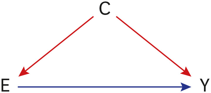
By definition, a confounder is a variable that influences both the treatment (exposure) and the outcome (Fig. 1, variable ‘C’ through the red paths), distorting the true association between the exposure and the outcome (Fig. 1, the blue path).5 For example, a health care provider that cares for large numbers of terminally ill patients may appear to provide poor-quality care if the outcome is going to be measured by “patient mortality.” Given that terminal conditions are commonly associated with an increased mortality rate, not taking the frequency of terminally ill patients receiving care (a confounding variable) into account would result in a biased estimate of the quality of care provided.

Fig. 1

Schematic representation of a confounder (‘C’). ‘E’ represents the exposure (treatment) and ‘Y’ is the outcome.

To have an unbiased estimate of the treatment effect from observational studies, it is necessary to identify the potential confounders and control for them. There are several common techniques used to identify and control for confounders. Different methods evaluate the association between the confounder and either the exposure (treatment) or the outcome and control for them.6 7 Herein, we present a bird’s eye view of the risk adjustment techniques commonly used in biomedical and health-related research.

RISK ADJUSTMENT

The outcome of interest in observational studies can commonly be affected by the a priori differences existing between the distribution of variables in the study groups. The differences may exist in the distribution of intrinsic patients’ attributes that cannot be modified (e.g., age and race), and the modifiable attributes such as the quality of the health care services provided and the diagnostic methods used. Many of these attributes (variables) may influence the outcome of interest, some may be confounders. Uneven distribution of these attributes among treatment groups may thus result in a biased estimate of the treatment effect. This bias could have vanished if the study participants had been randomized to the treatment groups. In mathematical parlance, we can write:

(Eq. 1)

Outcome = f (Intrinsic patients' attributes, Treatment effect, Random effect)

which means that the outcome is a function (represented by f) of intrinsic patients’ attributes (e.g., sex, race, and quality of care received), the treatment effect, and a random effect.8 The function could be as simple as a linear combination of the variables to more complicated functions. Risk adjustment methods are used to account for the “intrinsic patients attributes” (risk factors), to create the following equation:6

(Eq. 2)

Adjusted Outcome = f (Treatment effect, Random effect)

The adjusted outcome (expected outcome) is, therefore, only a function of the treatment effect and random effects—an unbiased measure of the treatment effect. Statistical methods will account for the random effects. Risk-adjustment is then a way to isolate the effect of the treatment (exposure) from that of other factors, such as the patient’s age and race, performance of the diagnostic tests used, or the severity of the disease, to name only a few.

Risk adjustment steps

The process involves five steps:

1) The researchers need to agree upon the outcome of interest. Examples of outcomes in health-related studies are mortality rate, hospital stay, and 5-year survival rate.

2) The variables potentially predicting the outcome of interest should be identified. Predictors commonly used in health-related research include age, sex, and history of prior illnesses. Choosing appropriate outcome predictors generally involves a thorough literature search and expert judgment.

3) Then, the predictors that the outcome should be adjusted for during the analysis should be identified. The choice of the risk factors is very important. The risk factor should be a good predictor of the outcome of interest, not a variable in the causal path, between the exposure (treatment) and the outcome (e.g., a complication). It should not include many variables so that its computation is easy. Having too many variables may also cause problems. For instance, the factor cannot be computed for many participants for lack of a single or more missing values.8

4) The next step is to operationalize the selected risk factors, which is commonly done by quantifying them. We may construct a new index from the scratch or preferably use an existing one. For example, APACHE (Acute Physiology, Age, Chronic Health Evaluation) III, a compound measure, is commonly used to predict the in-hospital death of patients admitted to intensive care units.9 EuroSCORE (European System for Cardiac Operative Risk Evaluation) is another compound score for prediction of operative mortality.10 Patient Management Category (PMC) Severity Scale is another example for a prognostic index for in-hospital morbidity and mortality.11

5) Combine the risk factors to construct a statistical model or another method of adjustment. The model constructed (mostly through multivariate regression models) combines the risk factors to give an estimate of the effect each of the risk factors exerts on the outcome of interest. The common models include linear regression, logistic regression, Poisson’s regression, and Cox regression models. An in-depth discussion of these models is beyond the scope of this review. Herein, we just present a brief description of each model.

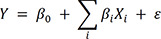
a) Linear regression model: This model is commonly used when the dependent variable (outcome) is continuous; independent variables can be continuous or categorical. In this model the dependent variable, Y, is a linear combination of independent variables, X:

(Eq. 3)
$Y = β_{0} + \sum_{i} β_{i} X_{i} + ε$

β represents the coefficients, reflecting the amount of change expected to occur in the outcome (Y) if the corresponding independent variable increases by one unit, keeping other independent variables constant; ε, the error term. When the dependent variable is dichotomous, binary logistic regression model is used.
b) Logistic regression model: In this model, the logit of the probability of the outcome of interest, P, is a linear combination of the independent variables, X:

(Eq. 4)
$l o g i t (P) = l n (\frac{P}{1 - P}) = β_{0} + \sum_{i} β_{i} X_{i} + ε$

The independent variables may be continuous or categorical. Herein, exp(β) is the odds ratio for the outcome happens if the corresponding independent variable increases by one unit, keeping other independent variables constant. As before, ε is the error term.
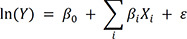
c) Poisson regression model is used when the dependent variable is a whole number of units or events in the model, the log-transformed of the dependent variable is a linear combination of independent variables, X:

(Eq. 5)
$l n (Y) = β_{0} + \sum_{i} β_{i} X_{i} + ε$

The mean and variance of the Poisson distribution are the same. When variance of an observed dataset is significantly higher than the measured mean, a situation termed “overdispersion,” then Poisson regression cannot be used; negative binomial regression should be, instead.
d) Cox regression model is a type of survival analysis where the dependent variable is time-to-event. The general equation of the Cox regression model is somewhat similar to Eq. 5, but the dependent variable is a function of time.

Performance of a model

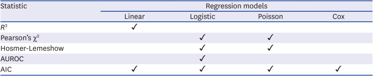
An important part of this approach is to evaluate the performance of the model constructed.6 There are several statistics for assessing the performance of the model (Table 1). Common examples are R², the coefficient of determination, which is the proportion of the variance explained by the model.12 Pearson’s χ² goodness-of-fit is another statistic used to determine whether the difference observed between the distribution of a categorical variable is significantly different from the expected distribution based on a given model.13 If the variable of interest is continuous, Hosmer-Lemeshow test is used instead.14 Area under the receiver operating characteristic (ROC) curve (the concordance or C-statistic) and Akaike Information Criterion (AIC) are other commonly used measures of the model performance.15 16 A comprehensive examination of these statistics is beyond the scope of this review.

Table 1

Statistics commonly used for evaluating the performance of a model and their applicability

Statistic	Regression models
Statistic	Linear	Logistic	Poisson	Cox
R²	✓
Pearson’s χ²		✓	✓
Hosmer-Lemeshow		✓	✓
AUROC		✓
AIC	✓	✓	✓	✓

AUROC = area under receiver operating characteristic curve, AIC = Akaike Information Criterion.

The methods described so far are widely used in biomedical and public health research. As an example, to adjust the risk of an unfavorable outcome in a series of Iranian patients with incidentally discovered liver hydatids, for a number of potential confounders, Saidi and Habibzadeh17 used a logistic regression model (the outcome was binary, “favorable” and “unfavorable”) to analyze their data collected in an observational study. In an attempt to determine the risk of tuberculosis among those immigrated to South Korea, Lee et al.,18 used a Poisson regression model to adjust the risk for potential confounders such as sex and age. In an ecological study we conducted to determine the effect of using oral polio vaccine as compared with inactivated polio vaccine on the cumulative number of cases diagnosed with COVID-19 (the dependent variable, which is a whole number), we used negative binomial regression (instead of Poisson regression, for overdispersion of the data) to adjust the risk for potential confounders.19 Finally, in a recent study, Jang et al.,20 used Cox regression analysis (in this survival analysis the dependent variable was time-to-death) to adjust the risk of 1-year mortality in patients from South Korea with COVID-19 for potential confounding variables.

Newer techniques

Although regression analysis methods described above can partly account for confounding variables, they may not always address the inter-group comparability.21 If many covariates are used in a multivariable regression analysis, the model may not have enough power to demonstrate a significant association between the outcome and the treatment; the results may even be misleading for overfitting.21 One of the methods commonly used to address this issue is matching of the study groups for important covariates.22 One of the most commonly used technique for matching is the propensity score matching.

Propensity score and propensity score matching

First described in 1983 by Rosenbaum and Rubin, propensity score analysis is one of the techniques that can be used for risk adjustment.23 The propensity score is the probability that a study participant receives a particular treatment. The probability is commonly computed using multivariable statistical methods, such as logistic regression model (Eq. 4), where the treatment of interest is the dependent variable; the covariates, independent variables. In the propensity score matching, the score is calculated for each study participant. Then, two groups of study participants—those who received the treatment of interest and those who did not—are created after matching individuals with similar propensity scores.21 24 In this way, the distributions of covariates in the two study groups are almost similar and the outcomes of the two groups are thus comparable, as if the study participants had been randomized.24 25 For propensity score matching, although no universally accepted threshold for standardized difference (i.e., the difference between the propensity scores of the two matched individuals divided by the pooled standard deviation) exists, a standard difference < 0.1 is often considered negligible.21 24 Unlike regression analysis, where to avoid overfitting including many covariates in the model is discouraged,21 including as many potential confounders as possible to develop the propensity score model is recommended.21 26 Many software programs can be readily used for propensity score matching (e.g., MatchIt package in R or the PSMATCH2 module in Stata^®).21 27 Many authors generally recommend that after the two study groups are matched using the propensity score matching, the outcomes observed in the two groups are better to be compared as if the data are paired—for example, by using Student’s t test for paired data to compare the two normally distributed continuous variables;28 Wilcoxon signed-rank test, two continuous variables not normally distributed;28 and the McNemar’s test, two categorical variables with binary outcomes.21 24 29

Target trial emulation

As mentioned above, randomization or conducting RCTs is not always possible or feasible. To determine the effect of a certain treatment on an outcome of interest, as if an RCT had been conducted, Hernán and Robins proposed in 2016 that it is possible to explicitly develop the protocol of a hypothetical RCT that would have answered the question. The technique is known as target trial emulation.30 This technique, which is really the application of the RCT study design in estimating the causal effect of an intervention based on the data collected from an observational study,31 has two main steps: 1) developing the protocol of the hypothetical RCT to articulate the causal question studied, and 2) explicitly emulating the components of the developed protocol given the data collected in the observational study.32

The protocol developed should include specific elements of the hypothetical RCT that define the inclusion/exclusion criteria, treatments available, assignment of participants to treatment arms, the start and end of follow-up, the outcomes of interest, causal contrasts (e.g., the intention-to-treat), and the data analysis plan.30 This hypothetical RCT then becomes the target study for the causal inference of interest. Note that it is very unlikely that the protocol includes information on blinded treatment assignment or outcome ascertainment because these are not commonly present in routine clinical practice.32

As a matter of fact, the target trial emulation is per se not able to eliminate the bias caused from lack of randomization in an observational study, even if all the emulated RCT protocol components were correctly considered to analyze the observational data. Detailed data on potential confounders are needed and necessary steps should be taken into account to control for confounders (e.g., by using propensity score matching of the study groups).32 The matching mimics the randomization that would have happened in the hypothetical RCT.

To better understand the method let us dissect a study conducted by Gupta et al., on the effectiveness of tocilizumab for the treatment of adults with COVID-19 admitted to intensive care unit (ICU).33 The data were collected for COVID-19 research studies conducted in 68 hospitals of the United States. At first, the authors described the protocol of a hypothetical RCT, the target trial, that could have been conducted to answer the research question. The authors defined the study population as adults with a positive COVID-19 laboratory test admitted to an ICU between March 4 and May 10, 2020 (the eligibility criteria). The adults were then supposed to be randomized (assignment to treatment arms) to receive tocilizumab or not (treatments available) within 2 days of their admission. The patients were then supposed to be followed until occurrence of in-hospital death, discharge, or termination of the trial on June 12, 2020 (the outcomes of interest). An intention-to-treat data analysis was supposedly used to compare the mortality between the study arms (causal contrasts and the data analysis plan).33 To emulate this target trial by using observational data, Gupta et al., identified 3,924 patients with laboratory-confirmed COVID-19 who met the inclusion and exclusion criteria and divided them into the treatment group (n = 433) who received tocilizumab, or the control group (those who did not receive tocilizumab within the first 2 days of ICU admission). To imitate the randomization in the hypothetical RCT, the authors used the propensity score analysis to control the effect of potential measured confounders.34 Another example is the study of Huh et al.,35 who conducted a target trial emulation to study the effect of oral antiviral agents on the risk of progression to severe COVID-19 in a group of patients aged 60 years or more in Korea.

Sometimes, we may use the technique without exclusively mention it (although this practice is not recommended). For instance, in a cohort study we conducted between March 20 and December 20, 2020, on almost 88,000 people, we practically used a target trial emulation design without exclusively mentioning that for the constraints imposed on the word count!36

In early 2020, when the COVID-19 was killing a large number of people across the globe, including Iran, and when we did not have ready access to an effective vaccine against the disease, we had a hypothesis that administration of oral polio vaccine, which contains live attenuated poliovirus, would confer temporary non-specific protection against COVID-19, probably through stimulation of the innate immunity. We designed an RCT, which was approved by the Ethics Committee of Shiraz University of Medical Sciences. However, permission to proceed with the trial was not granted by the Iran Food and Drug Administration. Simply put, in that trial, we supposed to randomize a group of adults into two groups, those who were supposed to receive a shot of oral polio vaccine and another group who did not receive the vaccine. At the end of study, presumably 6–9 months of participation, the cumulative incidence rates of COVID-19 in the two groups were compared. As we could not conduct the RCT, a cohort study was designed to emulate the target trial. After applying the inclusion and exclusion criteria, 9,270 women were found eligible to participate in the study, of whom 419 women were exposed to the live attenuated poliovirus. Propensity score matching was used to adjust the exposed and unexposed groups for several covariates and confounders. Of the remaining 8,851 unexposed women, 5,080 were excluded for not being matched with the 419 exposed women. This ensured that the two study groups were comparable as if the study participants had been randomized into two study arms. The outcome was time from the study participation to catching COVID-19 or study termination after 9 months. Using intention-to-treat principle, Cox regression analysis was employed to compare the outcomes measured in the two study groups (time-to-event) after adjusting for certain covariates.36 In this way, a cohort study was conducted to emulate a hypothetical RCT that could have not been conducted.

DISCUSSION

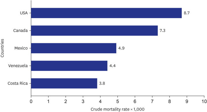
Risk adjustment is used to account for a priori differences existing in intrinsic patients’ attributes (usually beyond our control) when evaluating an outcome of interest. The method is commonly used in health-related studies. For example, if we examine the crude mortality rates in five North and South American countries in 1996 (Fig. 2), we can see that they are very different. Without accounting for confounders, one may interpret that the mortality rates in the United States and Canada are higher than those in Costa Rica, Venezuela, and Mexico. Although the reported numbers are correct, this analysis is misleading if the difference between mortality rates is construed as the difference in the health care status of the studied populations. Being associated with both the exposure (countries studied) and the outcome of interest (crude mortality rate), “age” is a confounder. The higher mortality rates in the United States and Canada are attributed to the differences in their population structure; both countries have a greater proportion of old people compared with other countries studied, presumably attributable to better health in these countries. Taking into account this issue and adjusting the mortality for age, the results will be very different.6

Fig. 2

Crude mortality rates measured in five countries in 1997. Reproduced from Arcà M, 2006.6

Apart from the broad range of applications of risk adjustment in research in general, this method is also widely used by health care agencies (e.g., Centers for Medicare and Medicaid Services) to ensure that the providers are paid fairly after adjusting for the intrinsic characteristics of the patient population they serve.37 In this way, the payments are modified according to the predicted expenditures derived from models based on the enrollee’s attributes such as demographic features and medical diagnoses, among other features.38 39 The final output of this model is a risk score scaled so that the population average equals one (i.e., normalization); values > 1 indicate higher-than-average risk and expected health care expenditure and vice versa. The adjusted payment to the provider will thus be calculated based on this score. This will provide an incentive for the health care providers to enroll all the beneficiaries irrespective of their demographics and medical conditions. This approach is also utilized to benchmark risk adjustment models and targets according to the patients’ health care status over time.37 40

In conclusion, risk adjustment methods are among the important statistical methods in the arsenal of health-related researchers and administrators. These methods have not only led to sound reasoning when assessing the association between an exposure and an outcome in epidemiological studies but have been widely used in health care systems to minimize costs and optimize outcomes. The methods are like the Swiss Army knives, complex and versatile, but they have their own limitations. Most of the models constructed for risk adjustment can only explain a relatively small proportion of the variance observed in the outcome of interest. Furthermore, different models constructed based on the very same dataset may lead to different judgments. For instance, authors of a study on stroke mortality rates in more than 9,000 patients from 94 hospitals, found that applying different models to the very same dataset gave very different results depending on which severity measure was used for risk adjustment.41 It is also noteworthy to consider that the explanatory power would be decreased when the number of risk adjusters included in a model is increased.42 In regression analysis, this is termed overfitting. Incorporating too many predictors in the model would result in fitting the noise instead of the signal. On the other hand, using a too simplistic model with just a few predictors would result in underfitting; it would result in missing important things. For instance, in linear regression, a linear relationship is assumed between the treatment and the outcome. This would be oversimplistic; in real world, variables correlate in a more complex way. These problems are not limited to regression models. Propensity score matching also assumes that all important confounders have been identified and included in the calculation of the propensity score. In reality, this is not necessarily true, and that is why the randomization cannot be totally replaced by propensity score matching. The matching technique is also sensitive to the method used for matching (the algorithm and the caliper choice). Likewise, target trial emulation has its own limitations. It can never replace RCTs. Emulating Leonardo da Vinci does not necessarily make one able to draw a masterpiece like Mona Lisa. Finally, it is of paramount importance that any risk adjustment processes used in health-related research studies should have a high degree of face validity among policymakers, administrators, and other end-users of the research to be considered credible. Some models, despite being constructed accurately, are very difficult to understand; clinicians and policymakers may be reluctant to accept them, and therefore, its implementation may be challenging.8

Notes

Disclosure: The authors have no potential conflicts of interest to disclose.

Author Contributions:

Conceptualization: Habibzadeh P, Habibzadeh F.
Data curation: Habibzadeh P, Habibzadeh F.
Formal analysis: Habibzadeh P, Habibzadeh F.
Investigation: Habibzadeh P, Habibzadeh F.
Methodology: Habibzadeh F.
Supervision: Habibzadeh F.
Validation: Habibzadeh P, Habibzadeh F.
Visualization: Habibzadeh P, Habibzadeh F.
Writing - original draft: Habibzadeh P, Habibzadeh F.
Writing - review & editing: Habibzadeh P, Habibzadeh F.

References

1. Broglio K. Randomization in clinical trials: permuted blocks and stratification. JAMA. 2018; 319(21):2223–2224. PMID: 29872845.

2. Zimmer WJ, Brown JT, Linzer M. Randomization in clinical trials. Ann Intern Med. 1987; 107(5):790.

3. Benson K, Hartz AJ. A comparison of observational studies and randomized, controlled trials. N Engl J Med. 2000; 342(25):1878–1886. PMID: 10861324.

4. Vandenbroucke JP. When are observational studies as credible as randomised trials? Lancet. 2004; 363(9422):1728–1731. PMID: 15158638.

5. Miettinen OS, Cook EF. Confounding: essence and detection. Am J Epidemiol. 1981; 114(4):593–603. PMID: 7304589.

6. Arcà M, Fusco D, Barone AP, Perucci CA. Risk adjustment and outcome research. Part I. J Cardiovasc Med (Hagerstown). 2006; 7(9):682–690. PMID: 16932082.

7. Rubin DB. Estimating causal effects from large data sets using propensity scores. Ann Intern Med. 1997; 127(8 Pt 2):757–763. PMID: 9382394.

8. Iezzoni LI. Risk Adjustment for Measuring Health Care Outcomes. 4th ed. Chicago, USA: Health Administration Press;2013.

9. Knaus WA, Wagner DP, Draper EA, Zimmerman JE, Bergner M, Bastos PG, et al. The APACHE III prognostic system. Risk prediction of hospital mortality for critically ill hospitalized adults. Chest. 1991; 100(6):1619–1636. PMID: 1959406.

10. Nashef SA, Roques F, Michel P, Gauducheau E, Lemeshow S, Salamon R. European system for cardiac operative risk evaluation (EuroSCORE). Eur J Cardiothorac Surg. 1999; 16(1):9–13. PMID: 10456395.

11. Young WW, Kohler S, Kowalski J. PMC Patient Severity Scale: derivation and validation. Health Serv Res. 1994; 29(3):367–390. PMID: 8063570.

12. Piepho HP. An adjusted coefficient of determination (R(2) ) for generalized linear mixed models in one go. Biom J. 2023; 65(7):e2200290. PMID: 37127864.

13. Chang S, Li D, Qi Y. Pearson's goodness-of-fit tests for sparse distributions. J Appl Stat. 2021; 50(5):1078–1093. PMID: 37009596.

14. Surjanovic N, Lockhart RA, Loughin TM. A generalized Hosmer-Lemeshow goodness-of-fit test for a family of generalized linear models. Test (Madr). 2024; 33(2):589–608. PMID: 38868722.

15. Habibzadeh F, Habibzadeh P, Yadollahie M. On determining the most appropriate test cut-off value: the case of tests with continuous results. Biochem Med (Zagreb). 2016; 26(3):297–307. PMID: 27812299.

16. Dziak JJ, Coffman DL, Lanza ST, Li R, Jermiin LS. Sensitivity and specificity of information criteria. Brief Bioinform. 2020; 21(2):553–565. PMID: 30895308.

17. Saidi F, Habibzadeh F. The non-operative management of asymptomatic liver hydatids: ending echinococcophobia. J Gastrointest Surg. 2018; 22(3):486–495. PMID: 29119531.

18. Lee YJ, Min J, Myong JP, Lee YH, Park YJ, Kim Y, et al. Incidence of tuberculosis among immigrants in Korea who participated in a latent tuberculosis infection screening program. J Korean Med Sci. 2024; 39(28):e207. PMID: 39048302.

19. Habibzadeh F, Chumakov K, Sajadi MM, Yadollahie M, Stafford K, Simi A, et al. Use of oral polio vaccine and the incidence of COVID-19 in the world. PLoS One. 2022; 17(3):e0265562. PMID: 35298546.

20. Jang Y, Hur HJ, Myung W, Park EJ, Park HY. Associations between COVID-19, delirium, and 1-year mortality: exploring influences on delirium incidence in COVID-19 patients. J Korean Med Sci. 2024; 39(32):e232. PMID: 39164056.

21. Yasunaga H. Introduction to applied statistics—chapter 1 propensity score analysis. Ann Clin Epidemiol. 2020; 2(2):33–37.

22. Iwagami M, Shinozaki T. Introduction to matching in case-control and cohort studies. Ann Clin Epidemiol. 2022; 4(2):33–40. PMID: 38504854.

23. Rosenbaum PR, Rubin DB. The central role of the propensity score in observational studies for causal effects. Biometrika. 1983; 70(1):41–55.

24. Haukoos JS, Lewis RJ. The propensity score. JAMA. 2015; 314(15):1637–1638. PMID: 26501539.

25. Loke YK, Mattishent K. Propensity score methods in real-world epidemiology: a practical guide for first-time users. Diabetes Obes Metab. 2020; 22 Suppl 3(S3):13–20. PMID: 32250525.

26. McCaffrey DF, Griffin BA, Almirall D, Slaughter ME, Ramchand R, Burgette LF. A tutorial on propensity score estimation for multiple treatments using generalized boosted models. Stat Med. 2013; 32(19):3388–3414. PMID: 23508673.

27. Zhao QY, Luo JC, Su Y, Zhang YJ, Tu GW, Luo Z. Propensity score matching with R: conventional methods and new features. Ann Transl Med. 2021; 9(9):812. PMID: 34268425.

28. Habibzadeh F. Data distribution: normal or abnormal? J Korean Med Sci. 2024; 39(3):e35. PMID: 38258367.

29. Austin PC. An introduction to propensity score methods for reducing the effects of confounding in observational studies. Multivariate Behav Res. 2011; 46(3):399–424. PMID: 21818162.

30. Hernán MA, Robins JM. Using big data to emulate a target trial when a randomized trial is not available. Am J Epidemiol. 2016; 183(8):758–764. PMID: 26994063.

31. Matthews AA, Danaei G, Islam N, Kurth T. Target trial emulation: applying principles of randomised trials to observational studies. BMJ. 2022; 378:e071108. PMID: 36041749.

32. Hernán MA, Wang W, Leaf DE. Target trial emulation: a framework for causal inference from observational data. JAMA. 2022; 328(24):2446–2447. PMID: 36508210.

33. Gupta S, Wang W, Hayek SS, Chan L, Mathews KS, Melamed ML, et al. Association between early treatment with tocilizumab and mortality among critically ill patients with COVID-19. JAMA Intern Med. 2021; 181(1):41–51. PMID: 33080002.

34. Xu S, Ross C, Raebel MA, Shetterly S, Blanchette C, Smith D. Use of stabilized inverse propensity scores as weights to directly estimate relative risk and its confidence intervals. Value Health. 2010; 13(2):273–277. PMID: 19912596.

35. Huh K, Jo Y, Bae GH, Joo H, Radnaabaatar M, Lee H, et al. Nationwide target trial emulation evaluating the clinical effectiveness of oral antivirals for COVID-19 in Korea. J Korean Med Sci. 2024; 39(42):e272. PMID: 39497563.

36. Habibzadeh F, Sajadi MM, Chumakov K, Yadollahie M, Kottilil S, Simi A, et al. COVID-19 Infection Among Women in Iran Exposed vs Unexposed to Children Who Received Attenuated Poliovirus Used in Oral Polio Vaccine. JAMA Netw Open. 2021; 4(11):e2135044. PMID: 34817583.

37. Risk Adjustment. Accessed June 20, 2024. https://www.cms.gov/priorities/innovation/key-concepts/risk-adjustment#:~:text=Risk%20Adjustment%3A%20A%20way%20to,the%20costs%20of%20those%20services .

38. Global and Professional Direct Contracting and Kidney Care Choices Models. Accessed June 20, 2024. https://www.cms.gov/priorities/innovation/media/document/dc-kcc-risk-adjustment-feb2022 .

39. Jacobs M, Morris E, Haleem Z, Mandato N, Marlow NM, Revere L. Drivers of individual and regional variation in cms hierarchical condition categories among florida beneficiaries. Risk Manag Healthc Policy. 2023; 16:1011–1022. PMID: 37323190.

40. Risk Adjustment Fact Sheet. Accessed June 20, 2024. https://www.cms.gov/medicare/medicare-fee-for-service-payment/physicianfeedbackprogram/downloads/risk-adjustment-fact-sheet.pdf .

41. Iezzoni LI, Shwartz M, Ash AS, Mackiernan YD. Predicting in-hospital mortality for stroke patients: results differ across severity-measurement methods. Med Decis Making. 1996; 16(4):348–356. PMID: 8912296.

42. Murtaugh CM, Peng T, Aykan H, Maduro G. Risk adjustment and public reporting on home health care. Health Care Financ Rev. 2007; 28(3):77–94. PMID: 17645157.