

 PDF
PDF ePub
ePub Citation
 Print
Print


I. Introduction
Sleep is a vital human need. Through sleep, physical and mental fatigue are relieved. Without adequate sleep, the ability to concentrate and participate in daily activities is decreased [1]. Research has shown that lack of sleep causes loss of strength, damages the immune system, and increases blood pressure [23]. Sleep disorders can be observed through examination of the sleep stage pattern.
Polysomnography is a tool to analyze the sleep pattern [456]. This test records physical activity when a person asleep. The test is essential as a first step to determine the type of sleep disorder. It combines electromyography (EMG), electrooculography (EOG), electrocardiogram (ECG), electroencephalography (EEG), and so forth. A doctor or health practitioner gives scores based on the data gathered. These scores are the gold standard in sleep stage analysis [78].
There are several techniques of sleep stage scoring, such as those developed by Rechtschaffen and Kales (R&K) and the American Academy of Sleep Medicine (AASM). The sleep stages are divided into two main categories, namely, rapid eye movement (REM), and non-rapid eye movement (NREM). In the R&K rules, NREM is divided into four stages: S1, S2, S3, and S4. The S3 and S4 stages can be categorized as slow-wave sleep (SWS). The delta waves comprise less than 50% of the total in S3 and more than 50% in S4. The S4 stage is the deepest among the NREM stages. REM sleep is the deeper than S4 and is often called the dream phase. The AASM rules refer to S1, S2, SWS, and REM as N1, N2, N3, and R.
A doctor or health practitioner takes several days to analyze data gather from a patient. Therefore, there is a need for an application that can automatically classify sleep stages. Several studies have developed machine learning algorithms for sleep stage classification. Aboalayon et al. [9] applied k-nearest neighbors, support vector machines (SVM), and neural networks. The research showed that SVM achieved the best performance. The success factor of SVM was its hyper-planes. Hassan and his colleagues [1011] performed the ensemble method. Some well-known algorithms for this purpose are boosting and random forest. At the beginning of boosting, all pieces of data have the same weight, but if a particular piece of data has not been classified, its weight is increased in the next iteration. The change in weight causes the data of the minor class to be modeled better. In the random forest method, trees are built, and classification is conducted through the voting of each tree [12]. The ensemble method is a good strategy to handle the class imbalance problem, which often occurs in sleep stage datasets. Langkvist et al. [13] proposed feature learning to achieve highly accurate sleep stage classification. They also implemented hidden Markov models (HMMs) for this purpose.
This paper proposes a new method based on feature learning called the fast convolutional method. It is one-dimensional (1D) convolutional, and this become the basis of its feature learning. It has an efficient running time and achieved through hierarchical softmax.
II. Methods
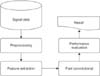
Figure 1 illustrates the process of the research design.
1. Signal Data
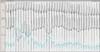
The dataset was obtained from the PhysioNet data center. The participants included 25 patients (21 men and 4 women) who had a sleep disorder. The patients were aged 28–68 years with body mass index scores ranging from 25.1 to 42.5 kg/m2, and their apnea-hypopnea index scores ranged from 1.7 to 90.9. The dataset recorded the movement of the rib cage, oronasal airflow, abdominal movement, snoring, and body position as well as readings obtained by EEG, EMG, EOG, and ECG. However, the PhysioNet data only included EEG, EMG, and EOG readings. The second dataset was obtained from Mitra Keluarga Kemayoran Hospital. Ten healthy respondents participated in this data collection. This study used EEG readings obtained from the Mitra Keluarga Kemayoran Hospital data. Example polysomnography signals are shown in Figure 2.
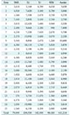
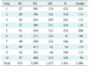
Every recording was divided into segments by using a 30-second window. An experienced sleep expert reviewed every segment and determined its score. The scoring of the PhysioNet data was based on R&K rules, and the Mitra Keluarga Kemayoran Hospital data was scored according to AASM rules. These scores became the ground truth for our system. Both datasets consisted of 5 labels. The number of segments for each sleep stage are shown in Tables 1 and 2. In the PhysioNet data, SWS and REM were the smallest, which means that the sick patients had difficulty getting deep sleep. In the Mitra Keluarga Kemayoran Hospital data, N1 was the smallest. In normal sleep patterns, N1 is a short stage of just 10 minutes.
2. Preprocessing
Preprocessing was conducted to get specific frequencies and amplify other frequencies. This process also reduced the data size without losing information. Notch and bandpass filters were applied to each segment. Notch filtering has the function of removing a single frequency from a signal [14]. This study removed a 50-Hz frequency from the signal at 128 Hz on the PhysioNet data, and at 200 Hz on the Mitra Keluarga Kemayoran Hospital data. The quality factor for the filter was set to 35. A bandpass filter passes a signal in the frequency range above the low-frequency limit (fL) and below the high-frequency limit (fH) [1516]. This study used fL = 0.3 for EEG and EOG, and 10 for EMG. Here, fH was the Nyquist frequency (sample rate/2). This result was then downsampled by two. It caused about 20% of the PhysioNet data and 15% of the Mira Keluarga Kemayoran data, out of the total dataset, to be removed.
3. Feature Extraction
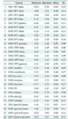
This process was conducted to extract the important feature to distinguish the characteristics of the sleep stages. This step produced 28 features of the PhysioNet data and 17 features of the Mitra Keluarga Kemayoran Hospital data. Tables 3 and 4 show the features.
The frequency domain was required to obtain the EEG signal information. Fast Fourier transform (FFT) was applied to convert the time domain to the frequency domain [17]. FFT utilizes the periodical properties of the Fourier transforms:

Here, yp(fb) is the sum of the absolute power of signal y in frequency band fb. The frequency bands are gamma (20–64 Hz), beta (13–20 Hz), alpha (8–13 Hz), theta (4–8 Hz), and delta (0.5–4 Hz).
The median is the middle value of a signal that has been sorted from the smallest to the largest value. If the amount of data is odd, then the median value is calculated as

However, if the amount of data is even, then the median corresponds to Equation (3):

This feature was used to obtain a representation of values that represent two EOG signals (left and right EOG).
Kurtosis is the level of precipitation of a distribution. The feature kurtosis was obtained to recognize the existence of K-complex. K-complex indicates that the data is categorized as S2. Its value is obtained by

where µ and σ are the average and standard deviation.
Entropy indicates the randomness of the signal distribution. The more random the distribution, the higher the entropy value. It also indicates signal complexity. The higher the entropy value, the more complex the signal. If a piece of data has a high entropy value, then it has a high probability to be categorized as S1 or REM:

where N is the number of samples in signal y, and nk is the number of samples of y belonging to the kth bin.
Each signal can be represented by the sum of sinusoids. Its representation is called the signal spectrum. It is often easier to analyze signals regarding spectral representation. The sinusoidal signal represented sleep spindles that indicated N2. The spectral mean value is calculated by

where F is the sum of the lengths of the 5 frequency bands.
Fractals are a geometric concept in which, if the objects are divided, the parts of the object will be similar to the original object. Its exponent value is calculated as the negative slope in the double logarithmic graph of the spectral density. In this study, if there was no fractal in the signal, then it was categorized as S1 or REM.
Dual-tree complex wavelet transform (DT-CWT) produces the same number of coefficients as the original signal. It is a variation of the discrete wavelet transform (DWT). DT-CWT uses 2 filter trees that represent the real and imaginary parts. The lost signal in the real part can be replaced by the imaginary part. The feature in this study helped to find the K-complex in the signal.
The features of the PhysioNet dataset were normalized by scaling, which made the signal size uniform. Then the under-sampling scheme was applied to handle class imbalance. Some stages had more data than the others. If this problem was not addressed, then the system tended to place each piece of data in the major class. This study implemented under-sampling based on the majority classes. This technique reduced the data in the major classes so that they were the same as the minority classes. The normalization and undersampling were conducted in accordance with method the proposed by Langkvist et al. [13] in testing the PhysioNet data.
4. Fast Convolutional Method
Both datasets show that sleep stage patterns appear on some adjacent data. This indicated that the classification model must be capable of capturing correlation among adjacent neighbors. The fast convolutional method does this by using a convolution layer, which is also useful to find the optimal features. The proposed method also had an efficient running time through hierarchical softmax. The softmax architecture is based on the Huffman coding tree [18]. Using this tree, softmax easily finds the class with the highest probability. The convolutional layer and hierarchical softmax are integrated and form the major parts of the proposed method.
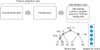
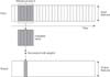
Our proposed method is shown in Figure 3. It consists of two primary layers, namely, the feature extraction and classification layers. The feature extraction layer is divided into two sub-layers: convolutional and pooling layers. The fast convolutional method applies a 1D convolutional layer, as shown in Figure 4 [19]. The input of the convolution layer is a 2D feature matrix, L × M. Here, L represents the length of the signal segments and M is the number of features. The window creates a new feature of the data.
At the convolutional layer, each neuron is locally connected to a small input area. All neurons with the same feature map obtain the data from different input areas. Then this layer correlates with some feature maps and also connects to the previous layer. The feature maps are obtained by the kernel. The calculation of the k-feature map ( ) uses the tanh function as follows:
) uses the tanh function as follows:
where Wk=weight, bk =bias.
The result of this convolutional layer becomes the input for the pooling layer, and it reduces the dimension of feature maps. The common strategies are max pooling and average pooling. The pooling layer divides the output of the convolution layer into several small grids. Then it takes the maximum or average value of each grid, respectively.
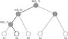
Its classification layer implements hierarchical softmax. This softmax enables fast calculation because it depends on fewer parameters. It uses a Huffman binary tree to represent sleep stages and the correlated features, as shown in Figure 5. A leaf represents the sleep stages, and the nodes are the features. For each leaf, there is a unique path from the root to itself, and this path is used to estimate the probability of a sleep stage.
The classification layer has two processes. First, it creates a Huffman tree based on features. Then we calculate the softmax value for each feature and sleep stage as

Here, fj is a function of every feature at j for z sleep stage, and k is the number of sleep stages. At the first iteration, its softmax value is calculated for each sleep stage. The feature and its sleep stage with the largest value become a winner pair. They have a high priority to be the main node and leaf. In the second iteration, two sub-processes are performed. The first sub-process calculates the softmax value based on the correlation between all features and the winning pair in the previous iteration. The second sub-process calculates the softmax value by computing all features to all sleep stages except the winning sleep stage. In this iteration, there are two winning pairs for each subprocess. The creation of new branches is stopped if all sleep stages have become leaves.
The second process of the classification layer is a prediction process. It is done by calculating softmax values between the data and all sleep stages based on the tree. Figure 5 illustrates the calculation of S2. The softmax value is only based on nodes in bold lines. The highest probability of a sleep stage becomes the prediction class. The fast convolutional method computes only the feature of the tree, not all features; thus, this method has a fast computation.
5. Performance Evaluation
The system was evaluated in terms of precision, recall, F-measure and running time. This study also implemented n-leave-one-out cross-validation, where n represents the number of pieces of data. The proposed method was compared with various machine learning models, such as Bayesian networks, naive Bayes, decision tree, k-nearest neighbors, random forest, bagging, and AdaBoost. We also compared the proposed method and DBN HMM on the PhysioNet data.
III. Results
The activation function in the convolutional layer of the fast convolutional method was based on a tanh function and max-pooling. The windows sizes were 15 in the PhysioNet data, and 3 in the Mitra Keluarga Kemayoran Hospital data. A total of 100 iterations were carried out using root-mean-square propagation as the optimizer. We also compared the proposed method with other machine learning models. The multilayer perceptron used the learning rate = 0.3, momentum = 0.2, and the hidden layers were (= number of features + 5)/2. The decision tree in this study was based on a C4.5 algorithm. The number of neighbors (k) in the k-nearest neighbor method was five. The base classifier of bagging was REPTree (Reduced-Error Pruning C4.5), and AdaBoost was decision stump. They wer conducted for 100 iterations.
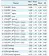
One important part of SVM is its kernel. This study applied a poly kernel in a multinomial logistic regression model as its calibrator. For comparison, the random forest method was conducted for 100 iterations. The performance of the proposed method was also compared with that of DBN HMM on the PhysioNet data. There were 200 hidden units for the 2 layers of DBN. The DBN had a function of quantization for HMM and was pre-trained for 200 iterations. The top layer used a softmax classifier for 50 iterations. Table 3 shows the results obtained by the proposed fast convolutional method and other methods. Precision, recall, and the F-measure were measured as percentages. The running time was measured in seconds (s). This study was conducted on a PC with Ubuntu 14.04 LTS 64, Hard Disk 240 GB, Four TITAN X GPUs with 12 GB of memory per GPU, Memory DDR2 RAM 64.00 GB, and Core i7-5820K CPU 3.3 @GHz.
IV. Discussion
This chapter discusses the results obtained by each algorithm with the two datasets. Table 5 shows the performance of each algorithm. AdaBoost showed the worst performance. Although it is an ensemble method, it failed to distinguish the stages. On the other hand, bagging and random forest achieved the best performance. The results showed that the decision stump in AdaBoost could not handle the complexity of the dataset. Unlike AdaBoost, the base classifier of random forest was a tree, so its performance was better. The use of resampling in the ensemble method, as well as bagging, also provided good performance. Thus, this algorithm achieved the best performance.
The second best performance was achieved by multi-layer perceptron. The use of multiple layers for feature learning successfully found the optimal feature for classification. This strategy was more effective than the use of hyperplanes in SVM. Naive Bayes had the lowest performance, which indicates that the features were not independent.
The machine learning models had F-measure results below 60% except for bagging and DBN HMM. DBN HMM is a sequence-based classifier. Its classification was not only determined by the features but also the interaction among stages. Both methods had the longest running times, which were more than 3,000 s. This means that it was not easy to get better performance with efficient running time. However, the fast convolutional method was able to do so. The algorithm had the highest F-measure for the PhysioNet data, taking just 42.58 s.
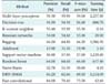
Table 6 presents the confusion matrix of the fast convolutional method for the PhysioNet data. The S2 stage was the most successfully classified. The second and third were S1 and awake, respectively. These stages were the majority classes in the PhysioNet dataset. On the other hand, REM and SWS were minority classes. They were the most challenging labels to be classified. The most difficult class to identify was REM. It was classified as S1 as much as 26.80% and as SWS 15.02%. This indicates that its model was not built well.
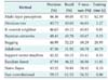
The fast convolutional method also performed well with the Mitra Keluarga Kemayoran Hospital data. Table 7 shows that the fast convolutional method had the highest F-measure of 56.32%. Unlike the PhysioNet data, the second highest F-measure was achieved by SVM. The hyper-planes were more needed than the ensemble models. The Mitra Keluarga Kemayoran Hospital data had a clear pattern because the respondents were healthy persons. Thus, hyper-planes could easily separate the stages. SVM needed 8.33 s for training its hyper-planes, which was an efficient running time. However, SVM was outperformed by the fast convolutional method in terms of both F-measure and running time. The fast convolutional models only required 0.06 s to be built.
This study used two different characteristic datasets. This difference was in the segment data distribution for each sleep stage. The data from the healthy participants had a clearer sleep stage pattern than the PhysioNet data. Although the same methods and parameters were used, the models of the machine learning methods for each dataset were different. This means that the chosen machine learning models must suit the characteristics of the dataset they are applied to. However, the proposed method showed good performance in terms of precision, recall, and F-measure for both datasets. It achieved the highest values compared to all machine learning models in this study. Its success can be attributed to its 1D convolutional layer. Its hierarchical softmax method in the classification layer also resulted in efficient running time. It can be concluded that the fast convolutional method is a promising tool for sleep stage classification.

 XML Download